数值数据集连列名都不一样，怎么让AI跨表检索、对齐？现有嵌入方法遇到异构表直接失灵，LLM也束手无策。 这个问题卡住了跨数据集RAG、算法选择、仿真初始化——没有共同特征名，相似性匹配只能靠猜。 论文提出：对每个表算20+统计描述符（均值、分位数、缺失率…），用sentence

---

Statistical Embeddings for Similarity, Retrieval, and Interpretable Alignment of Numeric Tabular Datasets

Source: https://arxiv.org/html/2605.30289 [1]\fnmM. Ross\surKunz

[1]\orgnameIdaho National Laboratory

Abstract

Numeric tabular datasets are the dominant data format in scientific practice, yet large language models lack native mechanisms for representing numeric datasets in a meaningful way across heterogeneous feature spaces. Existing approaches either target predictive modeling over individual datasets, which requires a shared set of variable definitions, or lack mechanisms for interpretable cross-dataset alignment. The proposed methodology characterizes numeric tabular datasets through structured exploratory data analysis descriptors, embeds those descriptors into a shared vector space using a pretrained sentence transformer, and quantifies cross-dataset similarity via Canonical Correlation Analysis (CCA). Furthermore, a penalized formulation of CCA is applied to recover sparse, interpretable variable-level correspondences between datasets, identifying which statistical descriptors or variable-level quantities drive cross-dataset alignment without requiring shared variable names or feature conventions. Differential privacy is optionally applied to the descriptor set prior to embedding, supporting deployment in sensitive data contexts without requiring access to raw observations at time of comparison. The methodology is evaluated across 15 datasets spanning general-purpose benchmarks, materials informatics, and nuclear-grade graphite characterization. Results demonstrate a totalP​@​1P@1score of 0.9, with known nearest-neighbor retrieval and cluster structure remaining robust across embedding ablations and differential privacy budgets. The proposed framework provides a principled pathway for integrating heterogeneous numeric data into retrieval-augmented generation pipelines while preserving statistical context, with direct applications to data-driven algorithm selection and simulation model initialization for unknown datasets.

keywords:

tabular data embedding, dataset similarity, canonical correlation analysis, retrieval-augmented generation

1Introduction

Numeric tabular datasets are the dominant data format in scientific practice, yet organizing, searching, and comparing such datasets across heterogeneous feature spaces remains a largely unsolved problem in data management and knowledge discovery. Scientific data repositories accumulate datasets that vary in sample size, variable composition, measurement scale, and domain context, making it difficult to determine which datasets are structurally related, which share distributional properties, or which are likely to respond similarly to a given modeling approach. Existing dataset search and profiling tools produce human-readable summaries or rely on schema matching over shared variable names, neither of which supports similarity comparison across datasets with disjoint feature spaces. This limitation is especially pronounced in natural science domains, where a single physical system may be characterized through multiple experimental modalities with incompatible variable definitions, and where the cost of redundant or mismatched modeling efforts is high. A principled representation of dataset-level statistical structure comparable across heterogeneous feature spaces, and interpretable in terms of the underlying data properties, would substantially advance the ability to organize, retrieve, and reason over large collections of scientific tabular data.

Large language model (LLM) embedding spaces offer a potential pathway toward such a representation. By encoding text into vectors of common dimension, pretrained sentence transformers enable similarity comparisons across documents from disparate domains without requiring shared vocabulary or structure. This capability motivates a statistical embedding strategy: rather than representing a dataset by its raw observations or variable names, one characterizes it through structured exploratory data analysis (EDA) descriptors, serializes those descriptors into natural language sentences, and embeds the resulting sentences into the LLM’s semantic space. The central challenge is ensuring that this embedding process preserves the statistical structure of the underlying data.

The proposed methodology computes individual statistical descriptors for each numeric column alongside multivariate summary quantities, which together serve as the basis for embedding tabular data into a shared vector space. These embeddings support hierarchical clustering and Canonical Correlation Analysis (CCA) across datasets, analogous to multi-view document embeddings[dhillon2011multi], even when data sources differ in dimension or variable composition. A penalized formulation of CCA is further employed to identify which variables or multivariate quantities drive cross-dataset correlation, yielding directly interpretable alignment structure. Differential privacy is optionally applied to the statistical descriptors prior to embedding, providing a principled mechanism for obfuscating sensitive summary information while preserving sufficient structure for meaningful cross-dataset comparison. Together, these components provide a means of interpretable tabular RAG that organizes heterogeneous numeric data while preserving statistical context.

The contributions of this work are as follows:

• •A structured EDA pipeline that produces statistically grounded, sentence-serialized descriptors for numeric tabular datasets, with optional differential privacy for sensitive data contexts, formalized as a mapping from a raw data matrix to a collection of embedding vectors in a shared semantic space.
• •A cross-dataset similarity framework based on mean canonical correlation between EDA embedding collections, supporting nearest-neighbor retrieval and hierarchical clustering across datasets with heterogeneous and disjoint feature spaces.
• •A penalized CCA formulation yielding sparse canonical loadings that identify which statistical descriptors or variable-level quantities drive cross-dataset alignment, providing interpretability not available under standard CCA.
• •Empirical validation across 15 datasets spanning general-purpose benchmarks, materials informatics, and nuclear-grade graphite characterization, demonstrating a totalP​@​1P@1score of 0.9 with nearest-neighbor retrieval.
• •A framework for retrieval-based algorithm and simulation model initialization, in which statistical similarity to cataloged datasets with known modeling outcomes supports data-driven selection of candidate methods for unknown datasets, connecting the proposed approach to meta-learning and AutoML pipelines.

The remainder of this paper is organized as follows. Section2reviews related work on tabular representation learning, dataset search, and differential privacy for data publishing. Section3describes the EDA fingerprinting pipeline, embedding procedure, and penalized CCA similarity framework. Section4details the datasets used for evaluation. Section5presents nearest-neighbor retrieval results, hierarchical clustering analysis, and penalized CCA interpretability examples. Section6summarizes the findings and discusses directions for future work.

2Related Work

2.1Tabular Representation and Foundation Models

Several lines of research have addressed the challenge of representing tabular data within learned model architectures. TabNet[arik2021tabnet]introduced sequential attention over tabular features to enable instance-wise feature selection during training, improving interpretability for prediction tasks. SAINT[somepalli2021saint]extended the transformer architecture to tabular data through inter-sample and inter-feature attention, demonstrating competitive performance on supervised learning benchmarks. TabPFNv2[hollmann2025accurate]demonstrated that a transformer pretrained exclusively on synthetic tabular data achieves state-of-the-art predictive accuracy on small datasets via in-context learning. TabICL[qu2025tabicl]extended this paradigm to large datasets through a two-stage column-then-row attention mechanism.[van2024tabular]argue that such Large Tabular Models (LTMs) remain significantly underrepresented in the foundation model literature despite the dominance of tabular data across scientific domains. Each of these approaches targets predictive modeling performance on individual datasets and does not address the problem of representing or comparing datasets across heterogeneous feature spaces.

2.2Dataset Search and Data Discovery

The problem of organizing and retrieving datasets from large repositories has received sustained attention in the data management community. Dataset search over data lakes, collections of heterogeneous raw data assets stored without imposed schema, has been formalized as a problem of identifying semantically or structurally related tables from among thousands of candidates[nargesian2019data]. A central challenge in this setting is that related datasets often share neither variable names nor schema structure, requiring similarity measures that operate over content rather than metadata alone. Schema matching approaches address this by identifying correspondences between column names or value distributions across pairs of tables[rahm2001survey], but these methods rely on lexical overlap or value-level comparison and do not generalize to datasets with entirely disjoint vocabularies. Dataset join and unionability discovery methods[zhu2019josie,nargesian2019data]extend schema matching to identify tables that can be joined or stacked, but again require overlapping values or column semantics and are not designed for cross-domain similarity assessment. The ARDA system[chepurko2020arda]and related augmentation frameworks treat dataset discovery as a feature engineering problem, identifying external tables that improve downstream model performance when joined to a query table, but this framing assumes a fixed target task rather than general-purpose similarity assessment. More recent work on dataset discovery for machine learning[zha2025data]has begun to treat datasets as first-class objects with learnable representations, but existing approaches remain largely confined to relational or structured tabular settings with compatible schemas. Existing profiling approaches produce human-readable summaries rather than embedding-compatible representations suitable for retrieval over heterogeneous collections.

2.3Tabular Retrieval-Augmented Generation and Embedding

Retrieval-augmented generation (RAG) offers a scalable approach to incorporating external knowledge at inference time by retrieving relevant context and injecting it into the model’s input[lewis2020retrieval]. Applied to tabular data, RAG pipelines retrieve relevant rows, columns, or dataset chunks at query time, but standard embedding models are pretrained predominantly on text corpora and underperform on numeric or relational table content. The Tabular Embedding Model (TEM)[khanna2025tabular]addresses this by fine-tuning lightweight embedding models specifically for tabular RAG pipelines, achieving substantial retrieval gains over general-purpose embedders. However, TEM operates at the row level within a single dataset and does not address cross-dataset similarity. The vision-language model connector paradigm[zhang2024vision,wu2019unified]demonstrates that heterogeneous modalities can be aligned into a shared latent space through learned projection modules, but[li2025lost]show that such projections distort local embedding geometry substantially. This geometric distortion finding motivates the use of distributional statistics rather than raw numeric values as the embedding substrate, as statistical descriptors are more naturally expressible in the semantic space of a pretrained sentence transformer than are raw numeric observations. No existing tabular RAG framework produces dataset-level embeddings that support cross-dataset similarity comparison while preserving interpretable statistical structure.

3Methodology

The proposed methodology is organized into two primary components. The first concerns the statistical characterization of numeric tabular datasets through a structured exploratory data analysis (EDA) framework. The second component addresses the transformation of these descriptors into a common vector space suitable for cross-dataset comparison and retrieval. Pairwise dataset similarity is then quantified through Canonical Correlation Analysis (CCA) with a sparse low dimensional approximation for interpretability.

3.1Problem Formulation

Let𝒟={X∈ℝn×p}\mathcal{D}=\{X\in\mathbb{R}^{n\times p}\}denote a numeric tabular dataset withnnobservations andppvariables. The goal is to construct a mappingϕ:𝒟→ℝd\phi:\mathcal{D}\rightarrow\mathbb{R}^{d}such that for a collection of datasets{𝒟1,…,𝒟N}\{\mathcal{D}_{1},\ldots,\mathcal{D}_{N}\}with potentially disjoint variable sets, the pairwise similaritys​(𝒟i,𝒟j)=f​(ϕ​(𝒟i),ϕ​(𝒟j))s(\mathcal{D}_{i},\mathcal{D}_{j})=f\!\left(\phi(\mathcal{D}_{i}),\phi(\mathcal{D}_{j})\right)reflects meaningful statistical relationships between datasets even whenpi≠pjp_{i}\neq p_{j}or the variable sets are entirely disjoint. The mappingϕ\phimust satisfy three properties. First, it must be computable without access to raw observations at comparison time, supporting privacy-preserving retrieval over sensitive data collections. Second, the resulting embedding must be compatible with a pretrained sentence transformer’s semantic space, enabling integration with downstream LLM-based retrieval pipelines. Third, the similarity measuressmust yield interpretable alignment structure that is recoverable via sparse canonical analysis, identifying which statistical descriptors or variable-level quantities drive cross-dataset correlation. Sections3.2and3.3describe the construction ofϕ\phiandssrespectively.

A common theme throughout the methodology is the use of penalized regression and matrix decomposition techniques, chosen primarily for interpretability. The unifying computational primitive is the singular value decomposition (SVD), which factorizes a data matrixX∈ℝn×pX\in\mathbb{R}^{n\times p}as:

X=U​Σ​V⊤,X=U\Sigma V^{\top},(1)whereU∈ℝn×rU\in\mathbb{R}^{n\times r}contains the left singular vectors,Σ∈ℝr×r\Sigma\in\mathbb{R}^{r\times r}is a diagonal matrix of ordered singular valuesσ1≥σ2≥⋯≥σr≥0\sigma_{1}\geq\sigma_{2}\geq\cdots\geq\sigma_{r}\geq 0,V∈ℝp×rV\in\mathbb{R}^{p\times r}contains the right singular vectors, andr=min⁡(n,p)r=\min(n,p)is the rank ofXX. Each application of the SVD in the proposed methodology serves a distinct interpretive purpose in different stages, e.g., imputation or cross-correlation between datasets. The general penalized regression problem that unifies these applications takes the form:

minβ⁡ℒ​(X,β)+∑jpλ​(|βj|),\min_{\beta}\;\mathcal{L}(X,\beta)+\sum_{j}p_{\lambda}(|\beta_{j}|),(2)whereℒ​(X,β)\mathcal{L}(X,\beta)is a loss function measuring fit to the data,β\betais the parameter vector of interest,pλp_{\lambda}is a penalty function controlled by regularization parameterλ>0\lambda>0, and the sum is taken over the components ofβ\beta. The choice ofℒ\mathcal{L}andpλp_{\lambda}can take on different forms depending on the application in the next subsections, e.g.,ℓ1\ell_{1}regularization for enforcement of sparsity. Together, these instantiations ensure that interpretability is preserved at every stage of the pipeline, from imputation through descriptor computation to cross-dataset alignment.

3.2Statistical Fingerprinting via EDA

Prior to dataset analysis, a lightweight structural assessment is performed to characterize the data matrix and guide downstream computation. LetX∈ℝn×pX\in\mathbb{R}^{n\times p}denote a numeric tabular dataset withnnobservations andppvariables. Missing values are tabulated across columns and imputed via soft-thresholding on the singular value decomposition[mazumder2010spectral]before any further computation is performed, as missingness in the raw matrix would otherwise corrupt the singular value spectrum used for rank estimation and multivariate characterization. Specifically, the imputed matrixX~∈ℝn×p\tilde{X}\in\mathbb{R}^{n\times p}is obtained by applying a soft-threshold operator to the singular values of the incomplete matrix, replacing missing entries with values consistent with a low-rank approximation. The numerical rank ofX~\tilde{X}is then estimated using the Gavish–Donoho optimal hard threshold[gavish2014optimal]. Lettingσmed\sigma_{\text{med}}denote the median of the observed singular values ofX~\tilde{X}, the thresholdτ^\hat{\tau}is given by:

τ^≈2.858⋅σmed,\hat{\tau}\approx 2.858\cdot\sigma_{\text{med}},(3)and the numerical rankr^\hat{r}is estimated as:

r^=∑k𝟏​[σk>τ^].\hat{r}=\sum_{k}\mathbf{1}[\sigma_{k}>\hat{\tau}].(4)Differential privacy is optionally applied at this stage to bound the sensitivity of subsequent summary statistics, ensuring that aggregate descriptors do not expose individual observations[dwork2025differential]. For each scalar descriptordkd_{k}with global sensitivityΔk\Delta_{k}, whereΔk\Delta_{k}denotes the maximum change indkd_{k}due to the addition or removal of a single observation, Laplace noise calibrated toΔk/ϵ\Delta_{k}/\epsilonis added prior to sentence serialization. Hereϵ>0\epsilon>0controls the privacy budget, with smaller values providing stronger privacy guarantees at the cost of greater descriptor perturbation.

Multivariate analysis is then performed to characterize the global structure and variable relationships withinX~\tilde{X}. Matrix-level norms and spectral quantities of{σk}\{\sigma_{k}\}are computed to summarize the overall scale, energy, and dominant directional structure; for example, the spectral norm is defined as‖X~‖2=σ1\|\tilde{X}\|_{2}=\sigma_{1}, the largest singular value. A full list of multivariate measures is provided in the first column of Table11. Prior to multivariate analysis, pairwise Pearson correlations are evaluated across all numeric columns, and variables exceeding a collinearity threshold (e.g.,R2>0.95R^{2}>0.95) are removed to avoid redundancy and suppress dominant pairwise structure that would otherwise obscure smaller multivariate interactions. This yields a reduced column set𝒩∗⊆{1,…,p}\mathcal{N}^{*}\subseteq\{1,\ldots,p\}. Multivariate variable importance is subsequently estimated using smoothly clipped absolute deviation (SCAD) penalized regression[fan2001variable,breheny2011coordinate], witha=3.7a=3.7and penalty parameterλ\lambdaselected via cross-validation. SCAD is preferred overℓ1\ell_{1}-based alternatives such as LASSO[tibshirani1996regression]because its non-concave form reduces estimation bias and produces sparser solutions through the oracle property[fan2001variable]. SCAD is not a strict requirement and the variable selection technique may be substituted depending on the domain, provided the objective remains identification of characteristic variable correlation fingerprints.

Univariate statistical descriptors are computed for each numeric variable to characterize its marginal distribution and temporal or sequential behavior. This includes standard exploratory quantities such as bounds, central moments, vector norms, and quantile summaries, as well as information-theoretic measures including entropy; a full list is provided in the second column of Table11. Robust statistics, e.g., median and median absolute deviation, are computed alongside their classical counterparts to provide outlier-resistant summaries of location and spread. For variables with sequential structure, autocorrelation coefficients are estimated to quantify serial dependence, and the Fast Fourier Transform (FFT) is applied to identify dominant periodic components and characterize the frequency content of each column. Change point detection is applied to identify structural breaks in the mean, variance, and joint mean-variance behavior of each column, yielding segment-level summaries that capture non-stationarity[killick2012optimal]. Specifically, the PELT algorithm with a BIC penalty is used to detect mean, variance, and mean-variance shifts, implemented via thechangepointpackage in R[killick2014changepoint].

Categorical variables, identified through cardinality thresholding atκ\kappa, receive dedicated treatment that combines column-level discrete summaries with partition-level continuous analysis. Let𝒞={j:|unique​(X:,j)|≤κ}\mathcal{C}=\{j:|\text{unique}(X_{:,j})|\leq\kappa\}denote the set of categorical column indices and𝒩={1,…,p}∖𝒞\mathcal{N}=\{1,\ldots,p\}\setminus\mathcal{C}the numeric columns. For each categorical columnj∈𝒞j\in\mathcal{C}, column-level descriptors include the absolute and relative frequency distribution over observed levels, the modal category and its frequency, and the number of unique levels. Additionally, for each category levelccwith at least 30 observations, the full univariate and multivariate descriptor sets described above are recomputed within the subset{Xi,::Xi,j=c}\{X_{i,:}:X_{i,j}=c\}, providing distributional characterization of each sufficiently represented group. Category levels with fewer than 30 observations are excluded from partition-level analysis to ensure descriptor stability, as moment and quantile estimates are unreliable at small sample sizes. For datasets containing a class variable, the class column is treated as categorical regardless of its numeric encoding, and partition-level descriptors are computed for each class level meeting the sample size threshold.

Data segments identified through change point detection receive analogous treatment. For each contiguous segmentssidentified within a numeric column, both the multivariate and univariate descriptor sets are recomputed within the segment, allowing the method to represent local distributional structure that would otherwise be obscured by global summaries computed over the full variable range. Segment-level descriptors are serialized using the same natural language templates as the global descriptors, with the segment index appended to the variable name token to distinguish local from global summaries.

Each statistical descriptor produced by the analysis pipeline is paired with a natural language sentence that contextualizes the numeric quantity. These sentences follow structured templates calibrated to each measure; for example, a singular value threshold entry might read:

The optimal singular value threshold is 23.4378; singular values below this are considered noise under the Gavish–Donoho criterion.

while a distributional descriptor might read:

Kurtosis is 2.4103; the distribution is platykurtic with lighter tails than normal.

The variable name or column header is then prepended to the sentence to supply feature-level context. For example:

Variable: pressure. Measure: kurtosis. Response: Kurtosis is 2.4103; the distribution is platykurtic with lighter tails than normal.

For multivariate or matrix-level descriptors, where no single variable can be attributed, the variable name is replaced with the tokenmatrixto distinguish aggregate quantities from column-specific ones. Let𝒮={t1,t2,…,tM}\mathcal{S}=\{t_{1},t_{2},\ldots,t_{M}\}denote the resulting ordered collection of descriptor sentences, whereMMdenotes the total number of sentences produced by the pipeline and depends onpp,nn, the number of detected change point segments, and the number of categorical levels meeting the sample size threshold. The embedding of𝒮\mathcal{S}into a shared vector space is described in Section3.3.

Figure 1:Statistical characterization process flow for moving from raw data to embeddings.Algorithm 1EDA Fingerprinting and Sentence Serialization1:Data matrix

X∈ℝn×pX\in\mathbb{R}^{n\times p}; privacy flag

dp∈{true,false}\texttt{dp}\in\{\texttt{true},\texttt{false}\}; privacy budget

ϵ>0\epsilon>0(used only if

dp=true\texttt{dp}=\texttt{true}); correlation threshold

ρ∈(0,1)\rho\in(0,1); cardinality threshold

κ∈ℤ+\kappa\in\mathbb{Z}^{+}; minimum partition size

nmin=30n_{\min}=30 2:Ordered sentence collection

𝒮={t1,…,tM}\mathcal{S}=\{t_{1},\ldots,t_{M}\}, where

MMdenotes the total number of descriptor sentences produced by the pipeline

3:Tabulate missing value counts per column; impute via soft-thresholded SVD[mazumder2010spectral]to obtain

X~\tilde{X}, prior to all subsequent computation

4:Compute SVD of imputed matrix

X~≈U​Σ​V⊤\tilde{X}\approx U\Sigma V^{\top}, where

U∈ℝn×rU\in\mathbb{R}^{n\times r},

Σ∈ℝr×r\Sigma\in\mathbb{R}^{r\times r}, and

V∈ℝp×rV\in\mathbb{R}^{p\times r}; estimate numerical rank

r^\hat{r}via the Gavish–Donoho threshold[gavish2014optimal]

5:Identify categorical columns:

𝒞={j:|unique​(X:,j)|≤κ}\mathcal{C}=\{j:|\text{unique}(X_{:,j})|\leq\kappa\}; let

𝒩={1,…,p}∖𝒞\mathcal{N}=\{1,\ldots,p\}\setminus\mathcal{C} 6:if

dp=true\texttt{dp}=\texttt{true}then

7:Add Laplace noise

Lap​(Δk/ϵ)\text{Lap}(\Delta_{k}/\epsilon)to each scalar descriptor

dkd_{k}, where

Δk\Delta_{k}is the global sensitivity of

dkd_{k} 8:endif

9:// Multivariate Descriptors

10:Compute matrix-level norms and spectral quantities for

X~\tilde{X}(see Table11)

11:Compute pairwise Pearson correlations among

𝒩\mathcal{N}; remove columns exceeding

ρ\rhoto form

𝒩∗\mathcal{N}^{*}; estimate multivariate variable importance via SCAD[fan2001variable]over

X~∗\tilde{X}^{*} 12:// Univariate Descriptors

13:foreach column

j∈𝒩j\in\mathcal{N}do

14:Compute univariate descriptors for

X~:,j\tilde{X}_{:,j}(see Table11)

15:Apply PELT with BIC penalty to

X~:,j\tilde{X}_{:,j}for mean, variance, and joint mean-variance shifts[killick2014changepoint]; record segment boundary locations

16:endfor

17:// Categorical and Segment Descriptors

18:foreach categorical column

j∈𝒞j\in\mathcal{C}do

19:Compute frequency distribution, modal category, and unique level count for

X:,jX_{:,j} 20:foreach level

ccwhere

|{i:Xi,j=c}|≥nmin|\{i:X_{i,j}=c\}|\geq n_{\min}do

21:Recompute univariate and multivariate descriptors within

{X~i,::Xi,j=c}\{\tilde{X}_{i,:}:X_{i,j}=c\} 22:endfor

23:endfor

24:foreach segment

ssidentified by change point detectiondo

25:Recompute univariate and multivariate descriptors within segment

ss; append segment index to variable name token

26:endfor

27:// Sentence Serialization

28:Initialize

𝒮←[]\mathcal{S}\leftarrow[\,] 29:foreach descriptor

dkd_{k}with variable name or tokenmatrixdo

30:Instantiate natural language template for

dkd_{k}; produce sentence

tkt_{k}; append to

𝒮\mathcal{S} 31:endfor

32:return

𝒮\mathcal{S}

The statistical descriptor computation described in Algorithm1is implemented in themungeRpackage, an open-source R package providing modular utilities for numeric and general-purpose embedding of tabular datasets[kunz2026mungeR]. The package includes all descriptor functions, sentence serialization templates, and differential privacy wrappers.

3.3Embedding, Hierarchical Clustering, and CCA

Each descriptor sentencetk∈𝒮t_{k}\in\mathcal{S}produced by the fingerprinting pipeline is encoded into a fixed-length embedding vector using a pretrained sentence transformerℰ:𝒯→ℝdℰ\mathcal{E}:\mathcal{T}\rightarrow\mathbb{R}^{d_{\mathcal{E}}}, where𝒯\mathcal{T}denotes the space of text strings anddℰd_{\mathcal{E}}is the output dimension of the chosen model. In this study, theall-MiniLM-L6-v2model is used, which producesdℰ=384d_{\mathcal{E}}=384-dimensional embeddings and is publicly available through Hugging Face[wang2020minilm]. This choice is not prescriptive; any sentence transformer producing embeddings of consistent dimension may be substituted depending on computational constraints or domain requirements. The embedding collection for dataset𝒟i\mathcal{D}_{i}is defined as:

Φi=[𝐯1(i);⋯;𝐯Mi(i)]⊂ℝdℰ,𝐯k(i)=ℰ​(tk(i)),\Phi_{i}=[\mathbf{v}_{1}^{(i)};\cdots;\mathbf{v}_{M_{i}}^{(i)}]\subset\mathbb{R}^{d_{\mathcal{E}}},\quad\mathbf{v}_{k}^{(i)}=\mathcal{E}(t_{k}^{(i)}),(5)whereMiM_{i}denotes the number of descriptor sentences produced for𝒟i\mathcal{D}_{i}by Algorithm1. The collectionΦi\Phi_{i}is represented as an embedding matrixVi∈ℝdℰ×MiV_{i}\in\mathbb{R}^{d_{\mathcal{E}}\times M_{i}}formed by concatenating the columns,[𝐯1(i);⋯;𝐯Mi(i)][\mathbf{v}_{1}^{(i)};\cdots;\mathbf{v}_{M_{i}}^{(i)}]which serves as the basis for cross-dataset comparison.

Cross-dataset similarity is quantified by comparing embedding matrices using Canonical Correlation Analysis (CCA). Given two embedding matricesVi∈ℝdℰ×MiV_{i}\in\mathbb{R}^{d_{\mathcal{E}}\times M_{i}}andVj∈ℝdℰ×MjV_{j}\in\mathbb{R}^{d_{\mathcal{E}}\times M_{j}}, CCA identifiesr∗r^{*}pairs of canonical directions that maximize the correlation between the projected embeddings, yielding canonical correlationsρ1≥ρ2≥⋯≥ρr≥0\rho_{1}\geq\rho_{2}\geq\cdots\geq\rho_{r}\geq 0, wherer∗=min⁡(r^i,r^j)r^{*}=\min(\hat{r}_{i},\hat{r}_{j}). The scalar similarity between𝒟i\mathcal{D}_{i}and𝒟j\mathcal{D}_{j}is defined as the mean canonical correlation:

si​j=1r​∑l=1rρl,s_{ij}=\frac{1}{r}\sum_{l=1}^{r}\rho_{l},(6)and the corresponding distance isDi​j=1−si​jD_{ij}=1-s_{ij}, withDi​i=0D_{ii}=0. This pairwise computation is repeated across all(N2)\binom{N}{2}dataset pairs in the catalog to construct the distance matrixD∈ℝN×ND\in\mathbb{R}^{N\times N}, which is then used as the basis for hierarchical clustering. Ward D2 linkage is adopted, which can be modified based on the specific application, as the agglomeration criterion, producing a dendrogram𝒯\mathcal{T}that organizes the catalog by statistical similarity and supports efficient retrieval when a new dataset𝒟q\mathcal{D}_{q}is introduced.

To recover interpretable alignment between dataset embedding spaces, a penalized formulation of CCA is applied using the penalized matrix decomposition framework[witten2009penalized]. Anℓ1\ell_{1}norm penalty is imposed on the canonical weight vectorswi∈ℝdℰw_{i}\in\mathbb{R}^{d_{\mathcal{E}}}andwj∈ℝdℰw_{j}\in\mathbb{R}^{d_{\mathcal{E}}}, inducing sparsity in the solution. Specifically, the penalized CCA problem is:

maxwi,wj⁡wi⊤​Vi⊤​Vj​wjsubject to‖wi‖2≤1,‖wj‖2≤1,‖wi‖1≤λ,‖wj‖1≤λ,\max_{w_{i},\,w_{j}}\;w_{i}^{\top}V_{i}^{\top}V_{j}w_{j}\quad\text{subject to}\quad\|w_{i}\|_{2}\leq 1,\;\|w_{j}\|_{2}\leq 1,\;\|w_{i}\|_{1}\leq\lambda,\;\|w_{j}\|_{1}\leq\lambda,(7)whereλ>0\lambda>0is a sparsity penalty selected either via sample permutation or fixed by the practitioner. Because each dimension ofViV_{i}corresponds to a distinct descriptor sentencetk(i)t_{k}^{(i)}rather than an arbitrary linear combination of features, the nonzero entries of the sparse solutionwi∗∈ℝdℰw_{i}^{*}\in\mathbb{R}^{d_{\mathcal{E}}}andwj∗∈ℝdℰw_{j}^{*}\in\mathbb{R}^{d_{\mathcal{E}}}identify which specific descriptors or variable-level quantities drive cross-dataset correlation. This provides a degree of interpretability that is not available under standard CCA, where the rank-rrapproximation distributes weight across all embedding dimensions simultaneously. The penalized CCA problem is solved iteratively for components1,…,r1,\ldots,r, deflatingViV_{i}andVjV_{j}after each component by subtracting the rank-one contribution of each solved component prior to estimating the next.

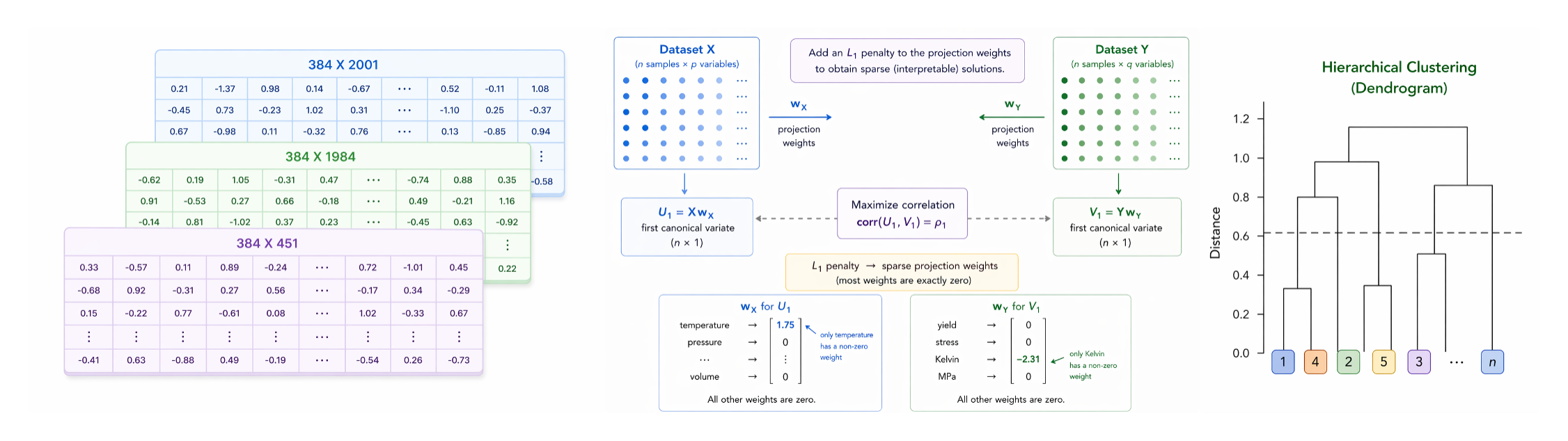Figure 2:Interpretable embedding process flow for determining data similarities.Algorithm 2Embedding, CCA Similarity, Retrieval, and Interpretable Alignment1:Sentence collections

{𝒮1,…,𝒮N}\{\mathcal{S}_{1},\ldots,\mathcal{S}_{N}\}from Algorithm1for catalog datasets

{𝒟1,…,𝒟N}\{\mathcal{D}_{1},\ldots,\mathcal{D}_{N}\}; query collection

𝒮q\mathcal{S}_{q}for new dataset

𝒟q\mathcal{D}_{q}; sentence transformer

ℰ:𝒯→ℝdℰ\mathcal{E}:\mathcal{T}\rightarrow\mathbb{R}^{d_{\mathcal{E}}}; number of neighbors

k∈ℤ+k\in\mathbb{Z}^{+}; linkage

ℓ\ell; interpretability flag

pcca∈{true,false}\texttt{pcca}\in\{\texttt{true},\texttt{false}\}; penalty

λ>0\lambda>0(if

pcca=true\texttt{pcca}=\texttt{true})

2:Top-

kkneighbors of

𝒟q\mathcal{D}_{q}; distance matrix

D∈ℝN×ND\in\mathbb{R}^{N\times N}; dendrogram

𝒯\mathcal{T}; sparse weights

{(wi∗,wj∗)}\{(w_{i}^{*},w_{j}^{*})\}(if

pcca=true\texttt{pcca}=\texttt{true})

3:// Embedding

4:foreach

𝒮i\mathcal{S}_{i},

i=1,…,Ni=1,\ldots,Nand query

𝒮q\mathcal{S}_{q}do

5:Encode each

tk∈𝒮it_{k}\in\mathcal{S}_{i}via

ℰ\mathcal{E}; stack rows to form

Vi∈ℝdℰ×MiV_{i}\in\mathbb{R}^{d_{\mathcal{E}}\times M_{i}} 6:endfor

7:// Pairwise CCA Similarity and Distance Matrix

8:foreach pair

(i,j)(i,j)with

1≤i<j≤N1\leq i<j\leq Ndo

9:Mean-center and

ℓ2\ell_{2}-normalize

ViV_{i},

VjV_{j}; apply Tikhonov regularization

α=10−6\alpha=10^{-6} 10:Compute CCA; set

si​j=1r​∑l=1rρls_{ij}=\frac{1}{r}\sum_{l=1}^{r}\rho_{l}where

r=min⁡(Mi,Mj,dℰ)−1r=\min(M_{i},M_{j},d_{\mathcal{E}})-1; set

Di​j=Dj​i=1−si​jD_{ij}=D_{ji}=1-s_{ij} 11:endfor

12:Set

Di​i=0D_{ii}=0for all

ii 13:// Hierarchical Clustering and Retrieval

14:Apply hierarchical clustering to

DDwith linkage

ℓ\ell; produce

𝒯\mathcal{T} 15:foreach

𝒟i\mathcal{D}_{i}in catalogdo

16:Compute

dq​i=1−1r​∑l=1rρld_{qi}=1-\frac{1}{r}\sum_{l=1}^{r}\rho_{l}between

VqV_{q}and

ViV_{i} 17:endfor

18:Sort by

dq​id_{qi}ascending; return top

kkas nearest neighbors of

𝒟q\mathcal{D}_{q} 19:// Penalized CCA (conditional)

20:if

pcca=true\texttt{pcca}=\texttt{true}then

21:foreach dataset pair

(𝒟i,𝒟j)(\mathcal{D}_{i},\mathcal{D}_{j})do

22:Estimate

λ\lambdavia permutation if not specified[witten2009penalized]

23:Solve

maxwi,wj⁡wi⊤​Vi⊤​Vj​wj\max_{w_{i},w_{j}}w_{i}^{\top}V_{i}^{\top}V_{j}w_{j}s.t.

‖wi‖2,‖wj‖2≤1\|w_{i}\|_{2},\|w_{j}\|_{2}\leq 1,

‖wi‖1,‖wj‖1≤λ\|w_{i}\|_{1},\|w_{j}\|_{1}\leq\lambda; obtain

wi∗,wj∗∈ℝdℰw_{i}^{*},w_{j}^{*}\in\mathbb{R}^{d_{\mathcal{E}}} 24:Map nonzero indices of

wi∗,wj∗w_{i}^{*},w_{j}^{*}to descriptor sentences and variable names

25:Deflate

ViV_{i},

VjV_{j}; repeat for components

2,…,r2,\ldots,r 26:endfor

27:endif

28:returntop-

kkneighbors;

DD;

𝒯\mathcal{T};

{(wi∗,wj∗)}\{(w_{i}^{*},w_{j}^{*})\}

4Experimental

4.1Experimental Setup

All experiments were conducted on an Apple MacBook Pro with an Apple M3 chip and 36 GB unified memory, running macOS. Statistical descriptor computation was performed in R using themungeRpackage[kunz2026mungeR]. Sentence embeddings were generated using theall\-MiniLM\-L6\-v2sentence transformer[wang2020minilm], accessed via thesentence-transformerpackage in Python[reimers-2019-sentence-bert], producing 384-dimensional embedding vectors for each descriptor sentence.

CCA was computed using the standard singular value decomposition formulation. To ensure numerical stability, embedding matrices were mean-centered andℓ2\ell_{2}-normalized prior to CCA computation. The number of canonical componentsrrwas set tomin⁡(Ri,Rj)\min(R_{i},R_{j})for each dataset pair, whereRiR_{i}andRjR_{j}denote the estimated numerical rank, via Gavish–Donoho, for datasets𝒟i\mathcal{D}_{i}and𝒟j\mathcal{D}_{j}respectively.

Penalized CCA was implemented using thePMApackage in R[witten2009penalized]. Penalty parameters were selected via sample permutation with 50 permutation replicates for the permutation-tuned condition, and fixed atλ=10−6\lambda=10^{-6}for the illustrative fixed-penalty condition. Initialization instability in the PMA coordinate descent algorithm was mitigated by running five random initializations per component and retaining the solution with the highest canonical correlation. Hierarchical clustering was performed using Ward D2 linkage via thehclustfunction in R. All random seeds were set to 42 throughout.

4.2Datasets

Three categories of datasets were selected for evaluation based on open-source availability and domain relevance: general-purpose benchmark datasets from the UCI Machine Learning Repository, steel and materials property datasets sourced from Citrine Informatics and the Materials Project, and nuclear-grade graphite characterization data maintained within the Nuclear Data Management and Analysis System (NDMAS) at Idaho National Laboratory. Summary statistics for each dataset are provided in the accompanying tables.

Three datasets from the UCI Machine Learning Repository[anderson1936species,fisher1936use,iris_53,heck1998corsika,magic_gamma_telescope_159,cortez2009modeling,wine_quality_186]were included to establish baseline performance on well-characterized benchmark datasets. The Iris dataset contains 150 specimens described by four morphological measurements (sepal length, sepal width, petal length, and petal width) across three species ofIris, making it a canonical low-dimensional classification benchmark. The Wine Quality datasets consist of separate red and white wine tables, each recording physicochemical properties such as acidity, residual sugar, chlorides, and sulfur dioxide levels alongside a sensory quality score; the red and white tables are treated as independent datasets in this work to preserve differences in their marginal distributions and sample sizes. The MAGIC Gamma Telescope dataset contains simulated high-energy gamma particle shower measurements recorded by an imaging atmospheric Cherenkov telescope, with features derived from the spatial and intensity distribution of the Cherenkov light pattern; the classification target distinguishes genuine gamma signal events from hadronic background events.

Four datasets characterizing the mechanical and physical properties of steels and inorganic materials were included to evaluate performance in a materials informatics context[agrawal2014exploration,citrination_agrawal,dunn2020benchmarking,citrination_mechanical_properties,ward2016general,de1988cohesion]. These datasets vary in size, feature construction strategy, and property target, providing complementary coverage of the materials property prediction problem. The Matbench steels and Citrine steels datasets originate from the same underlying experimental records; the Matbench version applies a standardized data cleaning and cross-validation protocol consistent with the broader Matbench benchmark suite, while the Citrine version represents the data in its original deposited form. Both are treated as separate entries to preserve this distinction.

Eight datasets characterizing nuclear-grade graphite were extracted from NDMAS at Idaho National Laboratory, as documented in[pham2025summary,NDMAS_Graphite]. The data support qualification of graphite grades for use as structural core components in high-temperature gas-cooled reactors (HTGRs). Specimens are drawn primarily from the 2114, IG-110, NBG-17, NBG-18, and PCEA grades, tested under both baseline (unirradiated) and irradiated conditions through the Advanced Graphite Capsule (AGC) irradiation program. Each of the eight NDMAS graphite datasets is treated as an independent tabular dataset, analyzed separately to reflect the practical scenario in which individual property tables are ingested and characterized without cross-table joins or shared identifiers.

A full list of the variables within each dataset is described in SectionSupplementary.

5Results

The experimental validation is organized into three subsections. Section5.1evaluates nearest-neighbor retrieval accuracy across embedding conditions and baseline methods, establishing whether the proposed EDA-derived embeddings recover meaningful dataset similarity structure at the individual dataset level. Section5.2expands this analysis to the full pairwise distance structure through hierarchical clustering, examining how embedding condition and differential privacy budget jointly affect the organization of the complete dataset collection. Section5.3demonstrates the interpretability of the framework through penalized CCA, identifying which statistical descriptors and variable-level quantities drive cross-dataset alignment for selected dataset pairs. Across all three analyses, results are reported for the full univariate and multivariate embedding condition, the multivariate-only ablation, and differentially private embeddings atϵ∈{0.1,1,10}\epsilon\in\{0.1,1,10\}.

5.1First neighbor relations and accuracy

A nearest-neighbor scheme analogous to document similarity is used to assess similarity between tabular datasets. Each dataset is compared to its nearest neighbor under several embedding conditions: the Uni/Multi-variate embedding (as described in the methodology); the Multivariate embedding, which summarizes univariate correlations, dimensionality, singular values, and multivariate responses; and differentially private embeddings at varying noise levels, whereϵ=0.1\epsilon=0.1corresponds to the highest noise injection andϵ=10\epsilon=10to the lowest. Results are organized by dataset group: Table4for the UCI Machine Learning datasets, Table4for the materials informatics datasets, and Tables4and4for the NDMAS graphite datasets. This section focuses on the nearest neighbor assignment; broader interpretation of embedding similarity is explored in Section5.3.

Among the UCI datasets (Table4), the red and white wine tables serve as a natural control pair, as both describe the same physicochemical feature space despite differing sample sizes. Considering them as a pair, theP​@​1P@1score, i.e., the correct top-1 nearest neighbors over all queries, results in a score of 0.90. The Iris and MAGIC Gamma Telescope datasets are included to characterize variation in nearest-neighbor assignment across less related datasets. Under the Multivariate embedding, the Iris and red wine datasets are assigned unexpected nearest neighbors relative to the other embedding conditions, suggesting that matrix-level summaries alone may not carry sufficient information to recover meaningful similarity. Across all other embedding conditions, Iris is consistently matched to IRRSummary, which is notable because if the similarity were driven purely by shared dimensionality, the Multivariate embedding would be expected to produce the same assignment. The telescope dataset exhibits the greatest instability in nearest-neighbor assignment across embedding spaces, reflecting its dissimilarity from the remaining datasets in this group.

Among the materials informatics datasets (Table4), the two Citrine datasets serve as a control pair, as both represent alloy compositions encoded as weight percentages. This pairing was recovered as mutual nearest neighbors across all embedding conditions, including atϵ=0.1\epsilon=0.1, demonstrating robustness to substantial noise injection and a perfectP​@​1P@1score. The Matbench steels dataset, which uses different units and measurement conventions than the Citrine steels dataset, is nonetheless correctly matched to Citrine steels in all conditions except the Multivariate embedding. Similarly, the Magpie and Miedema datasets span different feature spaces but share a common materials property description context, and are matched as nearest neighbors in all conditions except Multivariate resulting in aP​@​1P@1score of 0.8. The Miedema dataset shows the most variation within this group, with Tensile as its most frequent nearest neighbor outside the Magpie match; this may reflect the overlap in compressibility, shear modulus, melting point, and structural stability features shared between the two datasets.

Table 1:First nearest neighbors for the UCI Machine Learning datasets.Table 2:First nearest neighbors for the materials informatics datasets.Table 3:First nearest neighbors for the NDMAS datasets without ambient temperature and humidity variables.Table 4:First nearest neighbors for the NDMAS datasets with ambient temperature and humidity variables. The NDMAS nearest-neighbor results are presented in two tables (Tables4,4) separated by whether datasets include ambient temperature and humidity variables. Within the datasets lacking these variables (Table4), GasChem, IRRSummary, and SpecThermal are the most mutually similar, likely reflecting shared operational feature spaces including temperature, concentration, fluence, and displacements per atom (dpa). Under high obfuscation or Multivariate conditions, IRRSummary and GasChem are displaced toward Iris as a nearest neighbor, indicating that these embeddings no longer retain enough structure to resolve within-group similarity. Within the datasets containing ambient temperature and humidity (Table4), BulkDensity, Resistivity, Resonance, and SonicVelocity show overlapping nearest-neighbor assignments, particularly under obfuscation and Multivariate conditions. This cross-assignment pattern suggests that the full similarity structure within this group warrants examination of the complete similarity matrix, including hierarchical clustering, rather than nearest-neighbor summaries alone.

When considering all dataset pairs, i.e., red and white wines, citrine datasets, magpie connecting to miedema, and matbench steel to citrine steels, the totalP​@​1P@1retrieval accuracy score was 0.9.

5.2Hclust results

The previous section established that using only multivariate information or a high degree of obfuscation can introduce variation in nearest-neighbor assignment. This section expands on that analysis by examining the full pairwise distance structure,Di​jD_{ij}, across all datasets. Hierarchical clustering over these distances provides a means to identify which datasets should be grouped together and, more importantly, how cluster-level embeddings can support retrieval: a new dataset can be compared to the catalog by computing CCA between its embedding space and a cluster embedding space, rather than performing dataset-to-dataset comparisons.

Figure3compares hierarchical clustering results (Ward D2 linkage) across four embedding conditions. Subfigure3(a)uses the full univariate and multivariate descriptor set. Subfigure3(b)uses only multivariate descriptors, isolating the effect of excluding univariate content. Subfigures3(c)and3(d)progressively ablate contextual information from the sentence descriptors: first removing the statistic value (e.g., reducing “The median is 5.8. Variable: sepal.length” to the variable name alone), then also removing the variable name.

In the full univariate and multivariate dendrogram (Figure3(a)), the only unexpected grouping relative to the nearest-neighbor results is the pairing of the Miedema and telescope datasets, which is consistent with the high nearest-neighbor variability observed for both in Section5.1. When restricted to multivariate descriptors only (Figure3(b)), the cluster structure is largely preserved, with the primary change being that the red and white wine datasets are no longer directly linked, though they remain within the same cluster. Excluding the statistic value from the sentence descriptor (Figure3(c)) yields tighter grouping of the Magpie, Miedema, and telescope datasets relative to the full descriptor condition. Further excluding the variable name (Figure3(d)) produces a cluster structure visually similar to the full univariate and multivariate result, but with reduced inter-cluster separation as reflected in the dendrogram heights. Together, these results indicate that variable names and statistic values improve cluster resolution but are not required to recover the broad cluster structure, a property that is particularly relevant for datasets with nonstandard schemas or inconsistent naming conventions.

(a)Univariate and multivariate (b)Multivariate only (c)Univariate and multivariate, excluding statistic value (d)Univariate and multivariate, excluding statistic value and variable name

Figure 3:Hierarchical clustering (Ward D2) across four embedding conditions.The effect of differential privacy on cluster structure is examined in Figure4, which compares dendrograms across four privacy budgets using the full univariate and multivariate descriptor set. Recall thatϵ\epsiloncontrols the privacy budget, with smaller values providing stronger privacy guarantees at the cost of greater noise injection. Comparing the no-privacy baseline (Figure4(a)) to the lowest noise condition (ϵ=10\epsilon=10, Figure4(b)), the primary structural change is the migration of the Tensile, Compression, and Flex datasets toward closer association with Resonance and Resistivity, rather than with the operational parameter datasets GasChem and IRRSummary. To understand why specific dataset pairs are more susceptible to this structural displacement than others, Table5examines the spectral entropy of the singular value spectrum for a subset of NDMAS datasets across increasing levels of differential privacy noise, where spectral entropy serves as a measure of how uniformly variance is distributed across the directions of the data matrix. As the privacy budget decreases, the spectral entropy of Resonance and Resistivity converges toward that of Tensile, Compression, and Flex, while IRRSummary, GasChem, and SpecNeut remain near one. This convergence accounts for the dendrogram shifts observed for BulkDensity, Resonance, Resistivity, and SonicVelocity under obfuscation. More broadly, these results indicate that differential privacy budget selection will affect the similarity structure of datasets whose embeddings are dominated by variance descriptors; however, the overall cluster organization remains relatively stable, reflecting the inherent measurement noise present in the underlying data.

(a)No differential privacy (b)ϵ=10\epsilon=10 (c)ϵ=1\epsilon=1 (d)ϵ=0.1\epsilon=0.1

Figure 4:Hierarchical clustering (Ward D2) under varying differential privacy budgets.Table 5:Spectral entropy for a subset of NDMAS datasets under increasing differential privacy noise. As the privacy budget decreases, spectral entropy converges across datasets, shifting the similarity structure toward variance-dominated groupings.

5.3CCA results

To ensure interpretability of dataset associations, anℓ1\ell_{1}penalty is applied to the CCA calculation via penalized matrix decomposition. This yields sparse canonical loadings that identify the key variables contributing to each component. Three components are used here for demonstration; in practice, the number of components should be selected by examining the full cross-correlation structure.

Table7presents penalized CCA results between the two Citrine datasets, where the penalty parameter was selected via sample permutation[witten2009penalized]. Despite the two datasets using different units and column naming conventions (atomic percent vs. weight percent) to describe alloy composition, the first component recovers a shared set of alloying elements across the two representations. The specific elements selected do not correspond exactly by name, which warrants follow-up with a subject matter expert familiar with both datasets. The second component loads on multivariate matrix statistics in both datasets, which may reflect shared variance structure among the composition variables. The third component aligns on measures of mechanical strength, with fatigue strength in the Citrine Agrawal dataset corresponding to yield and ultimate tensile strength in the Citrine steels dataset. This is an encouraging result given that both studies examined the properties of steel compositions, and confirms that the penalized CCA recovers physically meaningful cross-dataset structure.

To illustrate the interpretability of penalized CCA more broadly, Table7presents results for three dataset pairs under a fixed penalty ofλ=10−6\lambda=10^{-6}: Citrine steel vs. Citrine Agrawal, Magpie vs. Miedema, and Tensile vs. Miedema. This fixed penalty is used for demonstration only; in practice the penalty should be optimized per dataset pair.

For the Citrine pair, restricting the penalty concentrates the first component on manganese content and the third component specifically on ultimate tensile and fatigue strength. For the Magpie and Miedema comparison, the first component links the number of elements to enthalpy of transformation, which have no direct physical relationship; however, the second component recovers a known correspondence between atomic weight and electron density, and the third component aligns molar volume across both datasets. The Tensile and Miedema comparison yields the most physically interpretable result: the first two components both align on elastic and shear modulus, and the third component relates pressure at fracture to melting point. These examples confirm that penalized CCA can surface interpretable cross-dataset variable correspondences even under a fixed, non-optimized penalty parameter.

Table 6:Penalized CCA results between the Citrine datasets. Theℓ1\ell_{1}penalty parameter was selected via permutation[witten2009penalized].Table 7:Non-zero canonical loadings from penalized CCA for three dataset pairs under a fixed penalty ofλ=10−6\lambda=10^{-6}. This penalty is illustrative; optimal selection should be performed per dataset pair.

6Conclusion

6.1Summary and Key Findings

This work introduced a framework for representing numeric tabular datasets as statistically grounded embeddings suitable for retrieval-augmented generation and cross-dataset comparison. The approach characterizes each dataset through a structured EDA pipeline that computes univariate and multivariate descriptors, serializes those descriptors into natural language sentences, and encodes them into a shared vector space via a pretrained sentence transformer. Pairwise dataset similarity is then quantified through CCA, with a penalized formulation providing sparse, interpretable canonical loadings that identify which specific variables or matrix-level quantities drive cross-dataset alignment.

Evaluation across 15 datasets spanning general-purpose benchmarks, materials informatics, and nuclear-grade graphite characterization demonstrated that the proposed embeddings recover meaningful similarity structure across substantially different domains and feature spaces. Nearest-neighbor retrieval achievedP​@​1P@1of 0.9 across all embedding conditions. Cluster structure was largely preserved under differential privacy noise, with perturbation effects concentrated among datasets whose embeddings are dominated by variance descriptors, as quantified through spectral entropy. Penalized CCA recovered physically interpretable cross-dataset correspondences without requiring shared variable names or feature conventions, including alignment of alloying elements across atomic and weight percent representations and correspondence of mechanical strength measures across independently constructed steel datasets. Together, these results demonstrate that EDA-derived statistical fingerprints provide a compact, semantically interpretable basis for organizing heterogeneous numeric data within LLM-compatible embedding spaces.

6.2Limitations and Future Work

Several limitations of the current framework warrant consideration. Embedding quality is bounded by the statistical content of the EDA descriptors, which summarize marginal and joint distributions but do not capture higher-order interactions or domain-specific structure falling outside the descriptor vocabulary. The sentence transformer used for encoding, all-MiniLM-L6-v2, was pretrained on general text corpora and has not been fine-tuned for statistical or scientific language; domain-adapted encoders may improve retrieval precision in specialized settings. The penalized CCA results presented here use fixed or permutation-selected penalty parameters applied uniformly across components, and a more principled cross-validated tuning procedure would strengthen the interpretability guarantees. Finally, the evaluation relies on nearest-neighbor and clustering metrics as proxies for retrieval quality; direct evaluation in an end-to-end RAG pipeline with downstream task performance would provide stronger empirical grounding.

A particularly promising direction for future work is the application of the proposed similarity measures to algorithm and model selection for unknown datasets, connecting the framework to the AutoML and meta-learning literature. In meta-learning, algorithm performance on a new task is estimated from the performance of candidate algorithms on similar prior tasks, with similarity typically defined over hand-crafted dataset meta-features such as dimensionality, class balance, and statistical moments[vanschoren2018meta,feurer2015efficient]. The EDA-derived embedding proposed here provides a richer and more principled characterization of dataset structure than existing meta-feature sets, and the CCA-based similarity measure offers a direct mechanism for identifying which prior datasets are most informative for warm-starting algorithm selection. In the AutoML context, this enables a retrieval-based initialization strategy: given an unfamiliar dataset, the nearest neighbors in embedding space identify candidate algorithms or hyperparameter configurations whose assumptions are most compatible with the observed statistical structure of the new data, reducing the search space before any model is trained. For example, a dataset whose fingerprint closely matches a known well-conditioned regression benchmark may be expected to support penalized linear models, while one resembling a high-dimensional materials informatics dataset with strong spectral concentration may be better suited to kernel or graph-based methods. Extending this paradigm to physics-based modeling and simulation, the same proximity structure could inform the selection of constitutive model forms, numerical solver settings, or simulation initialization parameters based on the statistical characteristics of empirical calibration data, connecting the framework to validated modeling and simulation workflows in scientific computing. This positions the proposed framework as a foundation for data-driven model recommendation systems that leverage accumulated institutional knowledge about algorithm and simulation performance across heterogeneous scientific datasets.

Acknowledgments

Work supported through the INL Laboratory Directed Research&\&Development (LDRD) Program under DOE Idaho Operations Office Contract DE-AC07-05ID14517. The authors of this work used Claude Sonnet 4.6 in the preparation of this document for general brainstorming and to improve grammar, sentence structure, and transitions. The authors have reviewed and take full responsibility for the resulting content.

References

Supplementary

6.3UCI Machine Learning Repository Datasets

6.3.1Iris (iris)

The Iris dataset contains 150 specimens across three species (Iris setosa,Iris versicolor, andIris virginica), with four continuous morphological measurements recorded per specimen[anderson1936species,fisher1936use,iris_53].

• •Variables:sepal.length, sepal.width, petal.length, petal.width, class

6.3.2MAGIC Gamma Telescope (telescope)

This dataset contains observations generated via Monte Carlo simulation of gamma-ray and hadron shower events recorded by an imaging atmospheric Cherenkov telescope[heck1998corsika,magic_gamma_telescope_159]. Continuous features describe the geometric and photometric properties of each shower image, and the binary response distinguishes signal (gamma) from background (hadron) events.

• •Variables:fLength, fWidth, fSize, fConc, fConc1, fAsym, fM3Long, fM3Trans, fAlpha, fDist, class

6.3.3Wine Quality (wine red and wine white)

The Wine Quality datasets consist of physicochemical measurements for red and white Vinho Verde wine samples from northern Portugal[cortez2009modeling,wine_quality_186]. The response is an ordinal quality score assigned by human sensory evaluation, commonly treated as either a regression or discretized classification target. The red and white subsets are treated as independent datasets in this work due to differences in composition profiles and class distributions.

• •Variables:fixed.acidity, volatile.acidity, citric.acid, residual.sugar, chlorides, free.sulfur.dioxide, total.sulfur.dioxide, density, pH, sulphates, alcohol, quality

Table 8:Dimensions of UCI Machine Learning Repository datasets.

6.4Steel and Materials Property Datasets

6.4.1Citrine Agrawal Steel Strength (citrine agrawal)

This dataset, hosted on the Citrination platform and introduced by[agrawal2014exploration,citrination_agrawal], was originally assembled from the National Institute for Materials Science (NIMS) public-domain database to support data-driven prediction of steel fatigue strength. Compositional and processing parameters serve as input features, and fatigue strength (MPa) is the regression target. Features span elemental composition fractions and thermo-mechanical processing conditions including reduction ratio, quenching temperature, and tempering temperature.

• •Variables:Normalizing Temperature C, Through Hardening Temperature C, Through Hardening Time min, Cooling Rate for Through Hardening C hr, Carburization Temperature C, Carburization Time min, Diffusion Temperature C, Diffusion Time min, Quenching Media Temperature for Carburization C, Tempering Temperature C, Tempering Time min, Cooling Rate for Tempering C hr, Reduction Ratio Ingot to Bar, Area Proportion of Inclusions Deformed by Plastic Work, Area Proportion of Inclusions Occurring in Discontinuous Array, Area Proportion of Isolated Inclusions, Fatigue Strength MPa, C at pct, Cr at pct, Cu at pct, Fe at pct, Mn at pct, Mo at pct, Ni at pct, P at pct, S at pct, Si at pct

6.4.2Citrine Steels (citrine steel)

This dataset contains mechanical property measurements for a collection of steel alloys described by elemental composition[citrination_mechanical_properties]. Feature representations are derived directly from alloy composition without additional processing parameters, and measured properties include yield strength, ultimate tensile strength, elongation, Charpy impact energy, and fracture toughness.

• •Variables:Yield strength YS MPa, Yield strength YS MPa temperature C, Ultimate tensile strength UTS MPa, Ultimate tensile strength UTS MPa temperature C, Elongation, Elongation temperature C, Charpy impact energy J, Charpy impact energy J temperature C, Fracture toughness KICMPa m, Fracture toughness KICMPa m temperature C, Al wt pct, C wt pct, Co wt pct, Cr wt pct, Mn wt pct, Mo wt pct, N wt pct, Nb wt pct, Ni wt pct, Si wt pct, Ti wt pct, V wt pct

6.4.3Matbench Steels (matbench steels)

The Matbench steels task is part of the MatBench v0.1 benchmark suite developed by the Materials Project for standardized evaluation of machine learning models on materials property prediction[dunn2020benchmarking]. The dataset contains 312 steel alloy compositions with yield strength (MPa) as the regression target, with features constructed from elemental composition strings spanning the full periodic table.

• •Variables:yield.strength, H, He, Li, Be, B, C, N, O, F, Ne, Na, Mg, Al, Si, P, S, Cl, Ar, K, Ca, Sc, Ti, V, Cr, Mn, Fe, Co, Ni, Cu, Zn, Ga, Ge, As, Se, Br, Kr, Rb, Sr, Y, Zr, Nb, Mo, Tc, Ru, Rh, Pd, Ag, Cd, In, Sn, Sb, Te, I, Xe, Cs, Ba, La, Ce, Pr, Nd, Pm, Sm, Eu, Gd, Tb, Dy, Ho, Er, Tm, Yb, Lu, Hf, Ta, W, Re, Os, Ir, Pt, Au, Hg, Tl, Pb, Bi, Po, At, Rn, Fr, Ra, Ac, Th, Pa, U, Np, Pu, Am, Cm, Bk, Cf, Es, Fm, Md, No, Lr, Rf, Db, Sg, Bh, Hs, Mt, Ds, Rg, Cn, Nh, Fl, Mc, Lv, Ts, Og

6.4.4MAGPIE (magpie)

The MAGPIE (Materials Agnostic Platform for Informatics and Exploration) feature set was introduced by[ward2016general]as a general-purpose descriptor framework for inorganic materials. MAGPIE defines a composition-based featurization scheme that computes statistics (mean, range, minimum, maximum, and mean absolute deviation) over 22 elemental properties for any stoichiometric formula, yielding a fixed-length numerical descriptor. In this work, MAGPIE features serve as the input representation for steel compositions drawn from the datasets described above, providing a physics-informed alternative to raw composition fractions.

• •Variables:MeltingT, Miracle Radius, Covalent Radius, First Ionization Energy, GSest FCClatcnt, Electronegativity, Density, ZungerPP.r s, Dipole Polarizability, GSest BCClatcnt, Log Thermal Conductivity, NsValence, GSmagmom, Polarizability, NValence, IsAlkali, AtomicVolume, phi, Number, IsNonmetal, NfValence, HHIp, VdWRadius, HHIr, Np Unfilled, Bulk Modulus, ZungerPP.r p, NsUnfilled, ZungerPP.r sigma, Thermal Conductivity, Atomic Radius, Shear Modulus, Is Metalloid, NfUnfilled, Second Ionization Energy, IsDBlock, Atomic Weight, Heat Vaporization, Mendeleev Number, GSvolume pa, NU nfilled, IsMetal, Electron Affinity, NdUnfilled, NdValence, MolarVolume, Column, ICSDVolume, IsFBlock, Space GroupNumber, Heat Capacity Mass, Allen Electronegativity, BoilingT, GSenergy pa, HeatCapacity Molar, n ws.third, HeatFusion, ZungerPP.r d, ZungerPP.r pi, NpValence, Row, Fusion Enthalpy, GSbandgap

6.4.5Miedema (miedema)

The Miedema dataset encodes binary alloy formation enthalpy estimates derived from the semi-empirical Miedema model[de1988cohesion], which characterizes intermetallic interactions through elemental parameters including electron density at the Wigner-Seitz cell boundary and electronegativity-related work function differences. These pairwise elemental descriptors provide thermodynamic context for alloy stability and are incorporated as supplementary features in the materials property prediction tasks examined here.

• •Variables:molar volume, electron density, electronegativity, valence electrons, a const, R const, H trans, compressibility, shear modulus, melting point, structural stability

Table 9:Dimensions of materials informatics datasets.

6.5NDMAS Graphite Datasets

6.5.1Bulk Density (BulkDensity)

Bulk density records in NDMAS are derived from dimensional and mass measurements collected as part of the baseline graphite physical properties characterization program. Specimen bulk density is computed from measured mass, diameter, and length, with geometry conforming to ASTM standard cylindrical specimen configurations.

• •Variables:amb temp, amb humidity, specimen length avg, specimen diam avg, mass, bulk density

6.5.2Compression (Compression)

Compressive strength measurements are obtained from cylindrical specimens machined to ASTM test standard geometries, capturing load, stress, displacement, and strain at maximum load.

• •Variables:amb temp, amb humidity, stress compr at max load, load compr at max load, displacement at max load, strain compr

6.5.3Flexure (Flex)

Flexural strength measurements are collected from specimens tested in three-point or four-point bending configurations per ASTM standard geometries, recording maximum load, maximum flexure stress, mid-span deflection, and elapsed time at peak load.

• •Variables:amb temp, amb humidity, pmaxflex, stress flex max, deflect mid at pmax, elapsed time at pmax

6.5.4Gas Chemistry (GasChem)

Records of gas composition captured during AGC irradiation campaigns characterize the helium purge environment surrounding irradiation capsules. These data serve as irradiation condition monitoring records rather than material property measurements.

• •Variables:CO2 Conc, CO Conc, Ar Conc

6.5.5Irradiation Summary (IRRSummary)

Summary records of irradiation conditions for AGC specimens include fast neutron fluence, irradiation temperature, and applied stress. These data provide the experimental context for interpreting post-irradiation property changes and are linked to the characterization datasets by specimen identifier.

• •Variables:AvgTemperature, CumeDoseDPA, PowerWgtedLoad

6.5.6Resistivity (Resistivity)

Electrical resistivity measurements are collected on graphite specimens prior to mechanical testing using standardized four-point contact methods per ASTM C611-05, providing a non-destructive characterization of the electrical transport properties of each specimen. Resistivity values are tightly distributed across specimens, reflecting the relatively uniform microstructural character of the nuclear-grade graphite grades tested.

• •Variables:amb temp, amb humidity, resistance, resistivity, potentialmeasure, AppliedCurrent, ComplianceVoltage

6.5.7Resonance (Resonance)

Resonance measurements characterize the elastic constants of nuclear-grade graphite specimens through fundamental frequency analysis in both flexural and torsional vibration modes, yielding dynamic Young’s modulus and shear modulus per ASTM C747-93 and ASTM C1259-08. The parallelepiped geometry of the flexural specimens is particularly well-suited for this measurement, providing accurate elastic constant determination from a single non-destructive test.

• •Variables:amb temp, amb humidity, resonance freq avg, elastic modulus flex

6.5.8Sonic Velocity (SonicVelocity)

Measurements of ultrasonic pulse velocity through graphite specimens serve as a non-destructive indicator of material condition and are used to derive elastic moduli including longitudinal, shear, and corrected elastic modulus alongside Poisson’s ratio.

• •Variables:vel sonic shear, elastic modulus long, elastic modulus shear, elastic modulus corrected, amb temp, amb humidity, poissons ratio

6.5.9Specimen Neutronics (SpecNeut)

Computed physics records for AGC specimens include fast neutron fluence and displacements per atom (dpa) derived from reactor physics calculations. These records quantify the radiation dose received by each specimen and serve as primary input variables for property change modeling.

• •Variables:Fluence, DPA

6.5.10Specimen Thermal (SpecThermal)

Specimen-level temperature records are derived from thermocouple measurements and thermal analysis of AGC capsule configurations, characterizing the thermal environment experienced by individual specimens during irradiation.

• •Variables:Temperature, ElevAboveMidCore

6.5.11Tensile (Tensile)

Tensile testing is performed on cylindrical dog-bone specimens per ASTM C749-08, capturing ultimate tensile strength, stress at break, strain at break, and elastic modulus for each specimen extracted from the graphite billet. Gauge diameters are verified against ASTM dimensional tolerances prior to testing, and extensometer-based strain measurements provide additional correlation with stress values through material elastic constants.

• •Variables:amb temp, amb humidity, stress rate, elastic modulus tensile, ultimate tensile strength, p at break, stress at break, strain1 at break, strain2 at break, strainavg at break

6.5.12Thermal Conductivity (ThermalConductivity)

Thermal diffusivity and thermal conductivity measurements are obtained from laser flash analysis on disk-shaped specimens per ASTM E1461-07. Thermal conductivity is particularly sensitive to radiation-induced lattice damage and is a primary design parameter for HTR core thermal analysis.

• •Variables:Temperature C, Thermal Conductivity W per mK

Table 10:Dimensions of NDMAS graphite datasets.

6.6Statistical Descriptors List

Table 11:Statistical descriptors computed at the multivariate and univariate level.