Deriving SVD without even aiming at it

# Connections in Math: deriving the SVD from scratch Source: [https://stillthinking.net/posts/connections-in-math-svd/](https://stillthinking.net/posts/connections-in-math-svd/) Disclaimer: no AI was used to write this\. Any errors, awkward sentences, and weird tangents are 100% organic, free\-range, and human\-made\. ## How to actually learn anything? For a long time I have always been asking myself what it really means to learn or grasp something in math\. I think this can be extended to other areas, but math is very often particularly distant from daily ordinary life when it comes to many of its concepts, and it’s hard for me \(at least\) to have an intuitive and natural understanding of it — the type of understanding that gives you some sort of foundational structure of the concepts and allows you to just reconstruct its details by yourself later in the future, with none or limited consultation\. I have experienced a few times this feeling of having really captured some sort of general structure in some areas, that allows me to express myself or deduce facts only consulting what I currently understand about it\. One good example is my first experience with Real Analysis\. At first, it looked very confusing and difficult, but after a while you capture some sort of structure of the main concepts and you can mostly run the concepts yourself\. But one thing took me too long to understand: traditional math books very often fail to give you a path that allows you to capture structure, or to grasp concepts in a more intuitive or natural way \(that would allow you to reconstruct it later\)\. This is because most math books present math in its final formalized version\. But they hide the path that was taken to get there: often messy, experimental, trial\-and\-error and tentative\. This blog assumes you already have basic knowledge in math\. It’s just not practical to teach everything from the ground up, but my goal is to write here some of the connections that helped me grasp concepts\. ## Starting Somewhere I’ve chosen to start from Linear Algebra \(L\.A\)\. It’s one of the most applicable and accessible areas in math\. When I was introduced to a central Linear Algebra concept called*Singular Value Decomposition*\(SVD\), it took me time to really understand what it is, and I think most books fail to explain it in a simple way simply because they usually start from the final conclusion formally stated, which makes no sense to the reader\. I think it’s critical to introduce motivation on why this was created in the first place\. Most things in applied math came from a specific problem someone was trying to solve\. Linear Algebra is a great place to start not only because it’s somehow simpler than more advanced non\-linear areas, but also because it’s connected to so many other areas, such as calculus, information theory, image processing, machine learning, and many others\. It’s some sort of basic or central area, although I think no matter where you start, if you continue to dig enough, you will reach connections to other areas — and in L\.A this is even more evident\. Let’s arrive naturally at SVD without even aiming at it\. The*matrix*of a Linear TransformationA\\mathbf\{A\}can be written differently for the same L\.T depending on the chosen input and output bases\. To see that, take a deliberately simple linear map — stretch thexx\-axis by 3, leaveyyalone: A\(x,y\)=\(3x,y\)\\mathbf\{A\}\(x, y\) = \(3x,\\ y\) In the**standard basis**, its matrix just reads off where the basis vectors land: M=\(3001\)M = \\begin\{pmatrix\} 3 & 0 \\\\ 0 & 1 \\end\{pmatrix\} Nothing could be clearer: “stretch one axis\.” Now describe the*same map*in a skewed basis: choose a slanted, non\-orthonormal basis: P=\(1112\),P−1=\(2−1−11\)P = \\begin\{pmatrix\} 1 & 1 \\\\ 1 & 2 \\end\{pmatrix\}, \\qquad P^\{\-1\} = \\begin\{pmatrix\} 2 & \-1 \\\\ \-1 & 1 \\end\{pmatrix\} The matrix of the same transformation in this basis isP−1MPP^\{\-1\} M P: P−1MP=\(2−1−11\)\(3001\)\(1112\)=\(54−2−1\)P^\{\-1\} M P = \\begin\{pmatrix\} 2 & \-1 \\\\ \-1 & 1 \\end\{pmatrix\} \\begin\{pmatrix\} 3 & 0 \\\\ 0 & 1 \\end\{pmatrix\} \\begin\{pmatrix\} 1 & 1 \\\\ 1 & 2 \\end\{pmatrix\} = \\begin\{pmatrix\} 5 & 4 \\\\ \-2 & \-1 \\end\{pmatrix\} Same transformation\. Same map on every actual vector\. But now it looks like an arbitrary tangle of scaling, shearing, and sign flips — you’d never guess it was just “stretchxxby 3\.” > The complexity was never in the map\. It was in the basis\. Sometimes we can*diagonalize*a matrix, by just choosing a new basis that makes the matrix ofA\\mathbf\{A\}diagonal \(this can only be done ifA\\mathbf\{A\}admits an Eigen Vector basis, but we will leave this fact unproved for now\)\. Of course, not all L\.T allow for a basis of Eigen Vectors\. In fact, some L\.T are not even square \(e\.g\. input dimension is not the same as output dimension\)\. We cannot even talk about Eigen Vectors for L\.Ts that don’t output to the same dimensional space, because an Eigen Vector stays fixed up to a scale, so it obviously restricts input and output to the same dimension\. When we**can**diagonalize a matrix, something interesting happens: we can clearly see that the Linear Transformation itself is basically a simple non\-uniform scale, disguised as something more complicated due to the basis chosen to represent the matrix \(the opposite of the operation we did before, where we showed a simple scale can be represented in a more complicated matrix form\)\. So we take the matrixMMof a diagonalizable L\.TA\\mathbf\{A\}, and write: M=P−1DPM = P^\{\-1\}DP and thenMMis*similar*to a diagonal matrix\. So the potentially complicatedMMis just a few numbers on the matrix’s diagonal and zeros everywhere else, up to a special change of basis matrixP\\mathbf\{P\}\. This is perfect for storing in a computer and to perform matrix multiplication efficiently\. We could convert our data to the reference frame ofP\\mathbf\{P\}once, make millions of matrix multiplications using a diagonal matrix \(easy\), then convert back to the original frame usingP−1\\mathbf\{P\}^\{\-1\}\. This simplification is possible because we could extract*structure*from the L\.TA\\mathbf\{A\}\. When do we fail to diagonalize a matrix? Well, if a diagonalizable matrix is just a disguised scale in some special coordinate frame, then we fail to diagonalize when the L\.T is anything more than a disguised scale \(actually, this is equivalent to saying thatA\\mathbf\{A\}cannot admit a basis of Eigen Vectors — try to prove that yourself\)\. For example, ifA\\mathbf\{A\}is a 2\-d rotation, it does not have two independent Eigen Vectors \(it has no*real*eigenvectors at all; a rotation moves every direction in the plane\!\)\. IfA\\mathbf\{A\}is a 2\-d shear, it surely cannot be diagonalized either, for a similar reason\. So can we still extract structure from just any L\.T in the same way we did with diagonalizable L\.Ts? If we could, then we might get some advantages, as we did with diagonal matrices… Intuitively, we can just look at what happens to anNN\-dimensional unit sphere through a generic L\.T: it can be non\-injective, that is, some directions might be annihilated \(collapsed to 0 — so a sphere would flatten into a disk\); it can scale other directions by an arbitrary value \(so a sphere or a disk would become an*ellipsoid*or*ellipse*\); it might rotate other directions by some arbitrary angle through arbitrary axes; it might also shear the sphere into other directions \(a sheared sphere is still a rotated ellipsoid\)\. This simple fact can be written as below: siui=Avis\_i\\, \\mathbf\{u\}\_i = \\mathbf\{A\}\\mathbf\{v\}\_i wheresis\_iis a*scalar*— the stretch factor — andui\\mathbf\{u\}\_iis a unit output direction\. That’s it\. We have detachedui\\mathbf\{u\}\_iandvi\\mathbf\{v\}\_i, and we don’t demand that they are Eigen Vectors anymore; they are just arbitrary vectors\. The expression above introduces no new fact, it’s just what happens to any L\.T, but it indeed captures our feeling that unit spheres are mapped to rotated ellipsoids in some way, if you seesis\_ias scale factors andui\\mathbf\{u\}\_ias the new rotated directions\. Our feeling now is that a L\.T might perform several types of operations \(rotation, shear, scale\) that, similarly to our diagonalization case, can possibly be decomposed and isolated, revealing some simpler structure in what initially seemed a complicated transformation\. As we saw earlier, skewed bases are not the best to represent a L\.T matrix, because they mix the coordinate basis vectors: each basis vector has a non\-zero projection onto the others\. The obvious next step here is to see what happens when the basesui\\mathbf\{u\}\_iandvi\\mathbf\{v\}\_iare orthonormal\. Can we always askui\\mathbf\{u\}\_iandvi\\mathbf\{v\}\_ito be orthonormal? We will see we can, and that’s an interesting and neat fact\. Look at what we are asking\. For the**output**vectors to be orthonormal: i≠j⟹<Avi,Avj\>=0,<Avi,Avi\>=1\(1\)\\tag\{1\} i \\neq j \\implies \\left<\\mathbf\{A\}\\mathbf\{v\}\_i, \\mathbf\{A\} \\mathbf\{v\}\_j\\right\> = 0, \\qquad \\left<\\mathbf\{A\}\\mathbf\{v\}\_i, \\mathbf\{A\} \\mathbf\{v\}\_i\\right\> = 1 and at the same time we want the**input**vectors to be orthonormal: i≠j⟹<vi,vj\>=0,<vi,vi\>=1\(2\)\\tag\{2\} i \\neq j \\implies \\left<\\mathbf\{v\}\_i, \\mathbf\{v\}\_j \\right\> = 0, \\qquad \\left<\\mathbf\{v\}\_i, \\mathbf\{v\}\_i\\right\> = 1 Now, something very interesting happens\. Rewrite the inner product of the outputs by movingA\\mathbf\{A\}to the other side \(using<Ax,y\>=<x,ATy\>\\left<\\mathbf\{A\}x, y\\right\> = \\left<x, \\mathbf\{A\}^T y\\right\>\): <Avi,Avj\>=<vi,ATAvj\>=viTATAvj\(1\.1\)\\tag\{1\.1\} \\left<\\mathbf\{A\}\\mathbf\{v\}\_i, \\mathbf\{A\}\\mathbf\{v\}\_j\\right\> = \\left<\\mathbf\{v\}\_i,\\, \\mathbf\{A\}^T\\mathbf\{A\}\\,\\mathbf\{v\}\_j\\right\> = \\mathbf\{v\}\_i^\{T\} \\mathbf\{A\}^T \\mathbf\{A\}\\, \\mathbf\{v\}\_j So far, nothing new — just rewriting the exact same expression\. But nowATA\\mathbf\{A\}^T \\mathbf\{A\}shows up explicitly, and it’s a symmetric matrix\! Take any \(potentially non\-square\) matrixCCand formCTCC^T C, and you will end up with a symmetric matrix\. Now, a very important fact here is that a symmetric matrix**always admits an orthonormal basis of Eigen Vectors**\(this is the spectral theorem\)\. So let us*choose*thevi\\mathbf\{v\}\_ito be exactly the orthonormal Eigen Vectors ofATA\\mathbf\{A\}^T\\mathbf\{A\}\. This immediately gives us \(2\), the input orthonormality, for free\. But here is the key point: this choice also gives us \(1\), the output orthogonality, automatically\. Watch what happens to the off\-diagonal casei≠ji \\neq j\. Sincevj\\mathbf\{v\}\_jis an eigenvector ofATA\\mathbf\{A\}^T\\mathbf\{A\}, we haveATAvj=λjvj\\mathbf\{A\}^T\\mathbf\{A\}\\,\\mathbf\{v\}\_j = \\lambda\_j \\mathbf\{v\}\_j, so: i≠j⟹<Avi,Avj\>=viTATAvj=λjviTvj=λj⋅0=0\(1\.2\)\\tag\{1\.2\} i \\neq j \\implies \\left<\\mathbf\{A\}\\mathbf\{v\}\_i, \\mathbf\{A\}\\mathbf\{v\}\_j\\right\> = \\mathbf\{v\}\_i^\{T\} \\mathbf\{A\}^T \\mathbf\{A\}\\, \\mathbf\{v\}\_j = \\lambda\_j\\, \\mathbf\{v\}\_i^\{T\} \\mathbf\{v\}\_j = \\lambda\_j \\cdot 0 = 0 The outputs are orthogonal precisely because the inputs were orthogonal eigenvectors ofATA\\mathbf\{A\}^T\\mathbf\{A\}\. We did not have to demand the output orthogonality separately — it fell out of the input choice\. And the lengths of those outputs are exactly the scale factors:<Avi,Avi\>=λi\\left<\\mathbf\{A\}\\mathbf\{v\}\_i, \\mathbf\{A\}\\mathbf\{v\}\_i\\right\> = \\lambda\_i, sosi=∥Avi∥=λis\_i = \\\|\\mathbf\{A\}\\mathbf\{v\}\_i\\\| = \\sqrt\{\\lambda\_i\}, and normalizing gives the orthonormal output directionsui=Avi/si\\mathbf\{u\}\_i = \\mathbf\{A\}\\mathbf\{v\}\_i / s\_i\. So we could not, in general, find an orthonormal basis thatA\\mathbf\{A\}itself diagonalizes — but we*can*always find one for the symmetric matrixATA\\mathbf\{A\}^T\\mathbf\{A\}, and that is exactly the input basis we were looking for\. ## The rank of A and the rank of AᵀA Another remarkable fact is that the*rank*ofA\\mathbf\{A\}is the**same**as the*rank*ofATA\\mathbf\{A\}^T \\mathbf\{A\}, and we will need it soon, so let’s prove it first\. ConsiderA:RN→RM\\mathbf\{A\}: \\mathbb\{R\}^N \\to \\mathbb\{R\}^M\. By the rank–nullity theorem, rank⁡\(A\)=N−dim⁡Ker⁡\(A\),\\operatorname\{rank\}\(\\mathbf\{A\}\) = N \- \\dim \\operatorname\{Ker\}\(\\mathbf\{A\}\), whereNNis the**input**dimension \(the kernel lives in the input spaceRN\\mathbb\{R\}^N\)\. Now notice thatATA\\mathbf\{A\}^T\\mathbf\{A\}isN×NN \\times N\(sinceAT\\mathbf\{A\}^TisN×MN\\times MandA\\mathbf\{A\}isM×NM\\times N\), so it also mapsRN→RN\\mathbb\{R\}^N \\to \\mathbb\{R\}^N, and the same rank–nullity theorem gives rank⁡\(ATA\)=N−dim⁡Ker⁡\(ATA\)\.\\operatorname\{rank\}\(\\mathbf\{A\}^T\\mathbf\{A\}\) = N \- \\dim \\operatorname\{Ker\}\(\\mathbf\{A\}^T\\mathbf\{A\}\)\. Both maps have the*same*domain dimensionNN, so to prove the ranks are equal it is enough to prove the kernels are equal: Ker⁡\(A\)=Ker⁡\(ATA\)\.\\operatorname\{Ker\}\(\\mathbf\{A\}\) = \\operatorname\{Ker\}\(\\mathbf\{A\}^T\\mathbf\{A\}\)\. **Proof\.** **\(1\)**First,Ker⁡\(A\)⊆Ker⁡\(ATA\)\\operatorname\{Ker\}\(\\mathbf\{A\}\) \\subseteq \\operatorname\{Ker\}\(\\mathbf\{A\}^T\\mathbf\{A\}\)— the easy direction: v∈Ker⁡\(A\)⟹Av=0⟹AT\(Av\)=0⟹v∈Ker⁡\(ATA\)\.\\mathbf\{v\} \\in \\operatorname\{Ker\}\(\\mathbf\{A\}\) \\implies \\mathbf\{A\}\\mathbf\{v\} = 0 \\implies \\mathbf\{A\}^T\(\\mathbf\{A\}\\mathbf\{v\}\) = 0 \\implies \\mathbf\{v\} \\in \\operatorname\{Ker\}\(\\mathbf\{A\}^T\\mathbf\{A\}\)\. **\(2\)**NowKer⁡\(ATA\)⊆Ker⁡\(A\)\\operatorname\{Ker\}\(\\mathbf\{A\}^T\\mathbf\{A\}\) \\subseteq \\operatorname\{Ker\}\(\\mathbf\{A\}\)— the less trivial direction\. At first it seems nothing stops a vectorv\\mathbf\{v\}that is*not*in the kernel ofA\\mathbf\{A\}from havingAv\\mathbf\{A\}\\mathbf\{v\}land in the kernel ofAT\\mathbf\{A\}^T, in which caseATAv=0\\mathbf\{A\}^T\\mathbf\{A\}\\mathbf\{v\} = 0even thoughAv≠0\\mathbf\{A\}\\mathbf\{v\} \\neq 0\. But it turns out this cannot happen\. SupposeATAv=0\\mathbf\{A\}^T\\mathbf\{A\}\\mathbf\{v\} = 0\. ThenAT\(Av\)=0\\mathbf\{A\}^T\(\\mathbf\{A\}\\mathbf\{v\}\) = 0, soAv∈Ker⁡\(AT\)\\mathbf\{A\}\\mathbf\{v\} \\in \\operatorname\{Ker\}\(\\mathbf\{A\}^T\)\. Two cases: - eitherAv=0\\mathbf\{A\}\\mathbf\{v\} = 0, sov∈Ker⁡\(A\)\\mathbf\{v\} \\in \\operatorname\{Ker\}\(\\mathbf\{A\}\)and we are done; - orAv≠0\\mathbf\{A\}\\mathbf\{v\} \\neq 0, which would put a*nonzero*vector in bothIm⁡\(A\)\\operatorname\{Im\}\(\\mathbf\{A\}\)\(sinceAv\\mathbf\{A\}\\mathbf\{v\}is, by definition, an output ofA\\mathbf\{A\}\) andKer⁡\(AT\)\\operatorname\{Ker\}\(\\mathbf\{A\}^T\)\. But this second case is impossible, because Im⁡\(A\)⊥=Ker⁡\(AT\)⟹Im⁡\(A\)∩Ker⁡\(AT\)=\{0\}\\operatorname\{Im\}\(\\mathbf\{A\}\)^\{\\perp\} = \\operatorname\{Ker\}\(\\mathbf\{A\}^T\) \\implies \\operatorname\{Im\}\(\\mathbf\{A\}\) \\cap \\operatorname\{Ker\}\(\\mathbf\{A\}^T\) = \\\{\\mathbf\{0\}\\\} \(a subspace and its orthogonal complement share only the zero vector\)\. SoAv=0\\mathbf\{A\}\\mathbf\{v\} = 0, i\.e\.v∈Ker⁡\(A\)\\mathbf\{v\} \\in \\operatorname\{Ker\}\(\\mathbf\{A\}\)\.■\\blacksquare A simpler, self\-contained way to prove this second direction is to use the positive\-definiteness of the inner product directly: ATAv=0⟹vTATAv=0⟹\(Av\)T\(Av\)=0⟹∥Av∥2=0⟹Av=0\.\\mathbf\{A\}^T\\mathbf\{A\}\\,\\mathbf\{v\} = 0 \\implies \\mathbf\{v\}^T\\mathbf\{A\}^T\\mathbf\{A\}\\,\\mathbf\{v\} = 0 \\implies \(\\mathbf\{A\}\\mathbf\{v\}\)^T\(\\mathbf\{A\}\\mathbf\{v\}\) = 0 \\implies \\\|\\mathbf\{A\}\\mathbf\{v\}\\\|^2 = 0 \\implies \\mathbf\{A\}\\mathbf\{v\} = 0\. The last step is exactly positive\-definiteness: only the zero vector has zero length\. Either route works; the first connects to the four fundamental subspaces, the second goes straight to the inner product\. Before assembling anything, let’s pause and list what we now know about*any*linear mapA\\mathbf\{A\}\(anM×NM \\times Nmatrix\)\. We set out to do for a general map what diagonalization did for the nice ones — extract structure — and it turns out we can extract quite a lot: - **Orthonormal frames on both sides\.**BecauseATA\\mathbf\{A\}^T\\mathbf\{A\}is symmetric, the spectral theorem hands us an orthonormal basis of input directionsvi\\mathbf\{v\}\_i\(its eigenvectors\)\. Pushing them throughA\\mathbf\{A\}and normalizing gives an orthonormal basis of output directionsui\\mathbf\{u\}\_i\. Both frames clean, no skew\. - **A rank that lines up\.**We provedrank⁡\(ATA\)=rank⁡\(A\)=r\\operatorname\{rank\}\(\\mathbf\{A\}^T\\mathbf\{A\}\) = \\operatorname\{rank\}\(\\mathbf\{A\}\) = r\. So exactlyrrof the eigenvaluesλi\\lambda\_iare nonzero, giving exactlyrrnonzero scale factorsσi=λi\\sigma\_i = \\sqrt\{\\lambda\_i\}\. The otherN−rN \- rinput directions are the kernel —A\\mathbf\{A\}sends them to zero\. - **A clean bijection in the middle\.**Thoserrsurviving input directions are linearly independent \(they are part of an orthonormal basis\), and they map torrlinearly independent output directions, one for one:Avi=σiui\\mathbf\{A\}\\mathbf\{v\}\_i = \\sigma\_i \\mathbf\{u\}\_i\. On the directions that matter,A\\mathbf\{A\}is just a clean, invertible scaling between two orthonormal frames — everything else it annihilates\. That last point is the heart of it\. Stripped of the kernel,A\\mathbf\{A\}does nothing exotic: it takesrrperpendicular input directions torrperpendicular output directions, stretching each by its own factorσi\\sigma\_i\. The “complicated transformation” was, once again, a simple scaling in disguise — we just needed*two*orthonormal frames instead of one to see it\. ## Collecting it into a factorization Now we collect theserrrelations into a single matrix equation\. Notice this is exactly the same relationsiui=Avis\_i\\, \\mathbf\{u\}\_i = \\mathbf\{A\}\\mathbf\{v\}\_iwe wrote down at the very start — only now we know thevi\\mathbf\{v\}\_iandui\\mathbf\{u\}\_ican be chosen orthonormal, and the scale issi=σi=λis\_i = \\sigma\_i = \\sqrt\{\\lambda\_i\}\. We have, one per surviving direction: Avi=σiui,i=1,…,r\\mathbf\{A\}\\mathbf\{v\}\_i = \\sigma\_i \\mathbf\{u\}\_i, \\qquad i = 1, \\dots, r with\{vi\}\\\{\\mathbf\{v\}\_i\\\}orthonormal in the input space and\{ui\}\\\{\\mathbf\{u\}\_i\\\}orthonormal in the output space\. Put thevi\\mathbf\{v\}\_ias the columns ofVrV\_r\(N×rN \\times r\) and theui\\mathbf\{u\}\_ias the columns ofUrU\_r\(M×rM \\times r\)\. ApplyingA\\mathbf\{A\}to each column ofVrV\_ris justAVr\\mathbf\{A\}V\_r, and the right\-hand side — eachui\\mathbf\{u\}\_iscaled byσi\\sigma\_i— isUrU\_rwith its columns scaled, which is exactly where the diagonalΣr\\Sigma\_rcomes from: AVr=\(∣∣σ1u1⋯σrur∣∣\)=\(∣∣u1⋯ur∣∣\)⏟Ur\(σ1⋱σr\)⏟Σr\\mathbf\{A\}V\_r = \\begin\{pmatrix\} \\vert & & \\vert \\\\ \\sigma\_1 \\mathbf\{u\}\_1 & \\cdots & \\sigma\_r \\mathbf\{u\}\_r \\\\ \\vert & & \\vert \\end\{pmatrix\} = \\underbrace\{ \\begin\{pmatrix\} \\vert & & \\vert \\\\ \\mathbf\{u\}\_1 & \\cdots & \\mathbf\{u\}\_r \\\\ \\vert & & \\vert \\end\{pmatrix\} \}\_\{U\_r\} \\underbrace\{ \\begin\{pmatrix\} \\sigma\_1 & & \\\\ & \\ddots & \\\\ & & \\sigma\_r \\end\{pmatrix\} \}\_\{\\Sigma\_r\} SoAVr=UrΣr\\mathbf\{A\}V\_r = U\_r \\Sigma\_r\. We are not collecting two matrices and then separately decomposing a third — the diagonalΣr\\Sigma\_r*appears on its own*, simply because scaling each column ofUrU\_rby its factorσi\\sigma\_iis the same as multiplyingUrU\_ron the right by a diagonal matrix\. The per\-direction scales collapse onto the diagonal for free\. To isolateA\\mathbf\{A\}, multiply on the right byVrTV\_r^T: AVrVrT=UrΣrVrT\.\\mathbf\{A\}\\,V\_r V\_r^\{T\} = U\_r \\Sigma\_r V\_r^\{T\}\. Here we must be careful:VrV\_rhas orthonormal*columns*, soVrTVr=IrV\_r^T V\_r = I\_r, butVrVrTV\_r V\_r^\{T\}is**not**the fullN×NN \\times Nidentity — it is the orthogonal projection onto the span of thevi\\mathbf\{v\}\_i\. That span is the row space ofA\\mathbf\{A\}, and its complement is the kernel, whichA\\mathbf\{A\}kills anyway\. So projecting it away changes nothing,AVrVrT=A\\mathbf\{A\}\\,V\_r V\_r^\{T\} = \\mathbf\{A\}, and we arrive at A=UrΣrVrT\\boxed\{\\ \\mathbf\{A\} = U\_r \\Sigma\_r V\_r^\{T\}\\ \} three width\-rrpieces: an orthonormal output frameUrU\_r, a diagonal of stretchesΣr\\Sigma\_r, and an orthonormal input frameVrTV\_r^T\. The same “extract the structure” move we made for diagonalizable maps — now done for*any*linear map at all\. ## The geometry behind it: the four subspaces We leaned on one fact in the rank proof — thatIm⁡\(A\)⊥=Ker⁡\(AT\)\\operatorname\{Im\}\(\\mathbf\{A\}\)^\\perp = \\operatorname\{Ker\}\(\\mathbf\{A\}^T\)— without really looking at it\. It is worth pausing on, because it carries a lot of geometric insight, and it explains*why*the kernel directions could be dropped so cleanly when we built the thin SVD\. A linear mapA\\mathbf\{A\}splits*each*of its two spaces into an**alive**part and a**dead**part\. In the input spaceRN\\mathbb\{R\}^N, the alive part is the row space \(the directionsA\\mathbf\{A\}actually acts on\) and the dead part is the kernel \(the directionsA\\mathbf\{A\}sends to zero\)\. In the output spaceRM\\mathbb\{R\}^M, the alive part is the image \(the directionsA\\mathbf\{A\}can reach\) and the dead part isKer⁡\(AT\)\\operatorname\{Ker\}\(\\mathbf\{A\}^T\)\(the directions no input ever maps onto\)\. And in both spaces,**the alive and dead parts are orthogonal**: RN=Row\(A\)⏟alive⊕Ker\(A\)⏟dead,RM=Im\(A\)⏟alive⊕Ker\(AT\)⏟dead\.\\mathbb\{R\}^N = \\underbrace\{\\mathrm\{Row\}\(\\mathbf\{A\}\)\}\_\{\\text\{alive\}\} \\oplus \\underbrace\{\\mathrm\{Ker\}\(\\mathbf\{A\}\)\}\_\{\\text\{dead\}\}, \\qquad \\mathbb\{R\}^M = \\underbrace\{\\mathrm\{Im\}\(\\mathbf\{A\}\)\}\_\{\\text\{alive\}\} \\oplus \\underbrace\{\\mathrm\{Ker\}\(\\mathbf\{A\}^T\)\}\_\{\\text\{dead\}\}\.  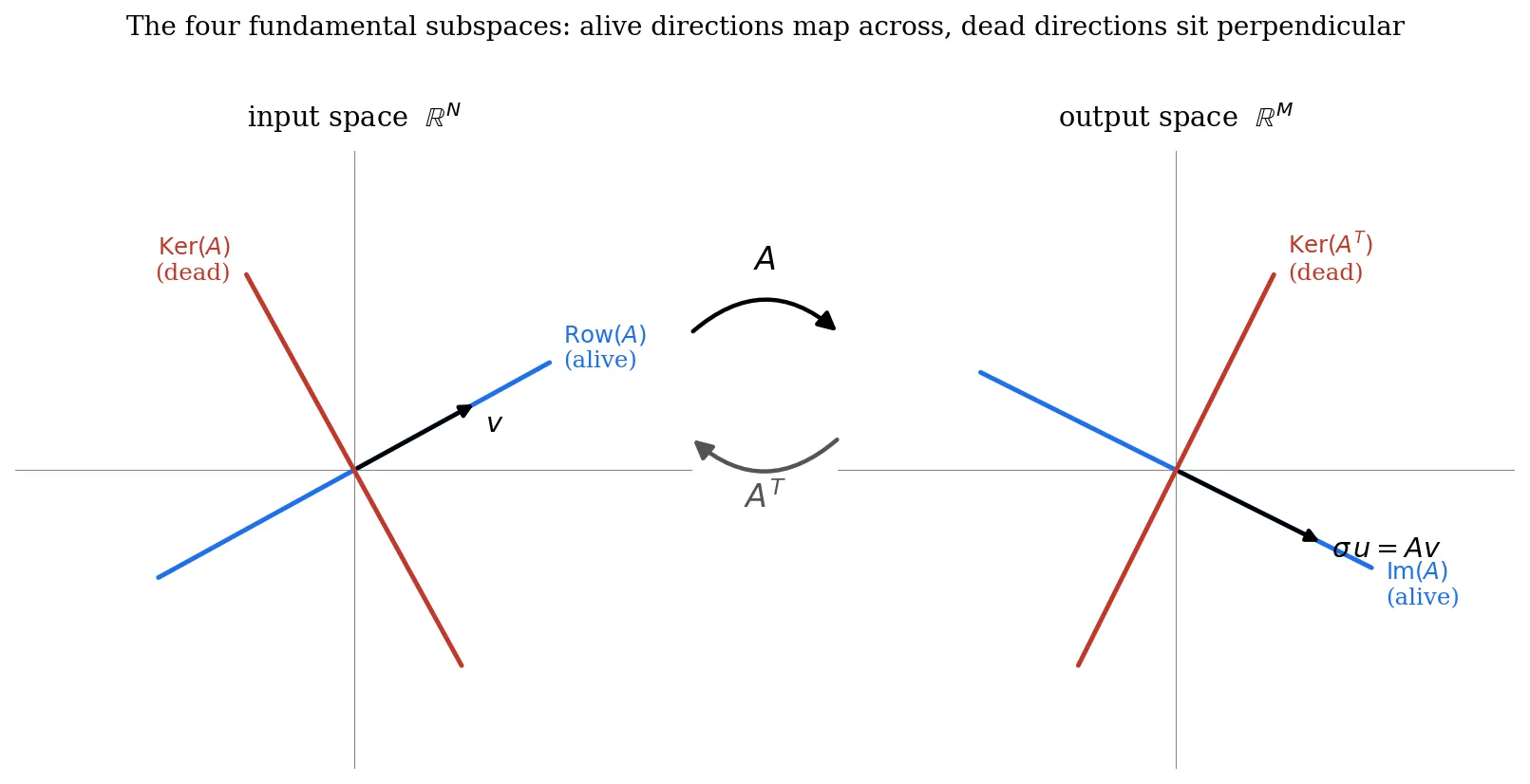Let me draw this in 2D, the simplest possible case\. In each space we have just two perpendicular lines: one alive, one dead\. Now here is the insight that makes the whole thing click\. Take a vectorv\\mathbf\{v\}sitting on the alive line of the input \(the row space\)\. ApplyA\\mathbf\{A\}: it lands on the alive line of the output \(the image\), stretched byσ\\sigma\. Now applyAT\\mathbf\{A\}^Tto bring it back\. CouldAT\\mathbf\{A\}^Tkill it? It could only kill a vector that lies inKer⁡\(AT\)\\operatorname\{Ker\}\(\\mathbf\{A\}^T\)— the*dead*output line\. But our vectorAv\\mathbf\{A\}\\mathbf\{v\}is on the*alive*output line, which is**perpendicular**to the dead one\. A vector sitting entirely on the alive line has*zero component*along the dead line\. So there is nothing forAT\\mathbf\{A\}^Tto annihilate — it carries the vector faithfully back to the input’s alive line\. That is the whole reason the round trip preserves the alive directions:**the dead direction is orthogonal to where the alive vectors live, so it cannot reach in and annihilate them\.**If the alive and dead parts were merely complementary but*skew*\(not perpendicular\), an alive vector could carry a sneaky component along the dead direction and lose it on the way through\. It is orthogonality — and only orthogonality — that keeps the alive subspace “pure”\. This is exactly why, when we built the thin SVD, dropping the kernel columns changed nothing: the kept directions and the discarded ones sit at right angles, so the discard touches nothing that matters\. ## A different way to write it: a sum of one\-dimensional pieces So far we wrote the SVD as a product of three matrices,A=UrΣrVrT\\mathbf\{A\} = U\_r \\Sigma\_r V\_r^T\. But there is a second way to read exactly the same equation that I find more revealing\. If you multiply it out, the product becomes a**sum**: A=∑i=1rσiuiviT\\mathbf\{A\} = \\sum\_\{i=1\}^\{r\} \\sigma\_i\\, \\mathbf\{u\}\_i \\mathbf\{v\}\_i^\{T\} Each termuiviT\\mathbf\{u\}\_i \\mathbf\{v\}\_i^\{T\}is an*outer product*: a column vector times a row vector, which produces a fullM×NM \\times Nmatrix — but a very special one\. It has**rank 1**: every column is a multiple ofui\\mathbf\{u\}\_i, every row a multiple ofvi\\mathbf\{v\}\_i\. It is the simplest possible non\-trivial matrix, a single “pattern”\. So the formula says something striking:*any*matrix is a**sum ofrrrank\-1 patterns**, each scaled by its singular valueσi\\sigma\_i\. The map is built by stackingrrone\-dimensional pieces on top of each other, from the strongest \(σ1\\sigma\_1\) to the weakest \(σr\\sigma\_r\)\. This also gives a clean second meaning to rank: it is the minimum number of rank\-1 pieces you need to build the matrix\. And it gives a meaning to the singular values that goes beyond “stretch factor”\. Order themσ1≥σ2≥⋯≥σr\>0\\sigma\_1 \\ge \\sigma\_2 \\ge \\dots \\ge \\sigma\_r \> 0\. A**large**σi\\sigma\_imeans that direction carries a lot of the matrix — it is a strong, genuinely present pattern\. A**small**σi\\sigma\_imeans that direction barely contributes; the matrix is*almost*the same without it\. Aσi\\sigma\_ithat is exactly zero means the direction contributes nothing at all \(it was never really there — it is the kernel\)\. So the singular value measures*how much that independent direction actually matters*to the matrix as a whole\. ## Throwing away the small pieces: compression Once you see the matrix as an ordered sum of rank\-1 pieces, an idea is irresistible: what if we keep only the first few? Define the**rank\-kktruncation**by keeping the topkkpieces and dropping the rest: Ak=∑i=1kσiuiviT,k<r\.\\mathbf\{A\}\_k = \\sum\_\{i=1\}^\{k\} \\sigma\_i\\, \\mathbf\{u\}\_i \\mathbf\{v\}\_i^\{T\}, \\qquad k < r\. This is a simpler matrix — fewer pieces, less to store — that*approximates*the original\. How good is the approximation? This is the beautiful part\. The**Eckart–Young theorem**says thatAk\\mathbf\{A\}\_kis the*best possible*rank\-kkapproximation ofA\\mathbf\{A\}: of all the matrices of rankkk, none is closer toA\\mathbf\{A\}\(in the least\-squares / Frobenius sense\)\. And the error you make is governed exactly by the singular values you threw away: ∥A−Ak∥F2=∑i=k\+1rσi2\.\\\|\\mathbf\{A\} \- \\mathbf\{A\}\_k\\\|\_F^2 = \\sum\_\{i=k\+1\}^\{r\} \\sigma\_i^2\. So the reconstruction error is just the sum of the squared*discarded*singular values\. If the smallσi\\sigma\_ireally are small, you can drop them and barely change the matrix — but you store far less\. This is**lossy compression**, and SVD tells you precisely the best way to do it and exactly what it costs\.  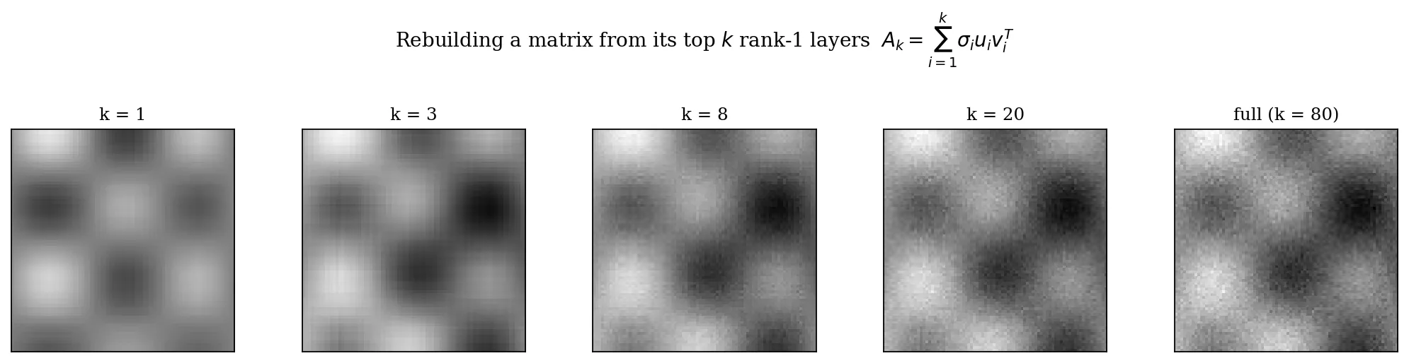Above, a single matrix \(think of it as an image\) rebuilt from its topkklayers\. Withk=1k=1you already see the dominant structure; byk=8k=8it is essentially there; the remaining dozens of pieces only add fine detail and noise\. We are not storing the whole matrix — we are storing a handful of strong patterns and discarding the long tail of weak ones\. Why does this work so well in practice? Because most real matrices are*compressible*: their singular\-value spectrum decays fast\.  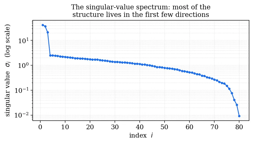The spectrum above drops off a cliff after the first few values\. That cliff is the matrix confessing that, although it is technically full of numbers, its*real*content lives in only a few directions\. The rest is redundancy\. ### The link to information and entropy This is where linear algebra quietly touches information theory, and it is the connection I find most satisfying\. Think of the squared singular valuesσi2\\sigma\_i^2as an “energy” carried by each direction\. Normalize them so they sum to one, pi=σi2∑jσj2,p\_i = \\frac\{\\sigma\_i^2\}\{\\sum\_j \\sigma\_j^2\}, and you have a*probability distribution*over directions — how the matrix’s energy is spread across its independent patterns\. Now the spectrum’s shape becomes a statement about*information*: - If a fewpip\_iare close to 1 and the rest near 0 \(a spiky distribution, low entropy\), the matrix is highly redundant — almost all its content is in a few directions, and it compresses dramatically\. - If thepip\_iare all roughly equal \(a flat distribution, high entropy\), the matrix is “incompressible” — every direction matters about the same, and there is nothing to throw away\. The**entropy of the singular\-value distribution**is, in this sense, a measure of how much genuine information the matrix carries versus how much is redundancy\. Compressing by truncating smallσi\\sigma\_iis exactly discarding the low\-probability, low\-information directions — the same move, in spirit, that lossy compression of any signal makes\. The singular values do not just decompose a transformation; they*rank its content by importance*, and importance is information\. ## Putting it to work We started by just trying to write a matrix in a simpler way, and we ended up with a tool that does a surprising amount: - **Compression\.**Keep the topkkrank\-1 pieces and you get the best possible low\-rank approximation, with a known, controllable error\. This is the engine behind image compression and low\-rank approximations everywhere\. - **Finding the directions that matter in data\.**If the rows ofA\\mathbf\{A\}are data points, the top singular directionsvi\\mathbf\{v\}\_iare the directions of largest variation in the data — the directions along which the data actually spreads\. This is**Principal Component Analysis**\(PCA\): it is just the SVD of the \(centered\) data matrix, andATA\\mathbf\{A\}^T\\mathbf\{A\}is, up to a scale, the covariance matrix whose eigenvectors we were computing all along\. Reducing dimensionality is then nothing but projecting onto the top fewvi\\mathbf\{v\}\_iand dropping the weak ones — the same truncation as compression, applied to data\. - **Understanding the map itself\.**The rank, the kernel, the image, the four subspaces — all of it can be read straight off the SVD: the rank is the number of nonzeroσi\\sigma\_i, the kernel is the directions withσi=0\\sigma\_i = 0, and the singular values tell you how the map stretches space\. And underneath all of these is a single picture, the one we built piece by piece:*every linear map takes an orthonormal set of input directions to an orthogonal set of output directions, stretching each byσi\\sigma\_i— a sphere becomes an ellipsoid\.*Compression is keeping the long axes of that ellipsoid\. PCA is finding them in data\. The four subspaces are the alive axes versus the flat ones\. They are all the same fact, seen from different sides — which, more than the formula itself, is the thing I wanted to capture here\. ## Where this goes next The entropy of the singular\-value spectrum gave us one kind of compressibility: it asked how a matrix’s*energy*is spread across its directions, and called something redundant when that energy piled into a few\. But that is a purely*statistical*notion — it sees how often things happen, never*why*\. So let me leave a puzzle that this view cannot answer\. Take two files of a million digits: one is random noise, the other is the first million digits ofπ\\pi\. Statistically they are indistinguishable — both look uniform, both “incompressible” by entropy\. Yet one you can send as a three\-line program and the other you cannot\. The next post chases exactly that gap: we will build Shannon entropy from scratch \(the same quantity we just used here\), watch it fail to notice the structure inπ\\pi, and follow that crack to*Kolmogorov complexity*— the length of the shortest program that reproduces an object — and the strange, beautiful fact that this truest measure of compression turns out to be provably**uncomputable**\. Statistical redundancy, it will turn out, is just the computable shadow of a deeper structure we can never fully pin down\.