Efficient AI Lecture 19: Distributed Training (Part 1)

This lecture gave me a much clearer picture of how self-attention parallelism actually flows across GPUs.

Start with the Transformer attention block: input tokens are projected into Q, K, V. In tensor parallelism, the QKV projections can be split across GPUs, often by attention heads. Each device computes only part of the projection. After local attention computation, the output projection needs synchronization. The partial outputs from different GPUs are combined with communication primitives such as All-Reduce. For long sequences, sequence parallelism changes the axis: instead of only splitting heads or hidden dimensions, we split the tokens across devices.

My note: https://ickma2311.github.io/ML/HW-SW-codesign/efficient-ai-lecture-19-distributed-training-part-1.html…

Distributed Training (Part 1) – ∇ ickma.dev

Source: https://ickma2311.github.io/ML/HW-SW-codesign/efficient-ai-lecture-19-distributed-training-part-1.html Distributed training is about splitting model training across devices while controlling two bottlenecks:

• **Memory:**can the model, gradients, activations, and optimizer states fit?
• **Communication:**can devices exchange tensors fast enough to keep compute busy?

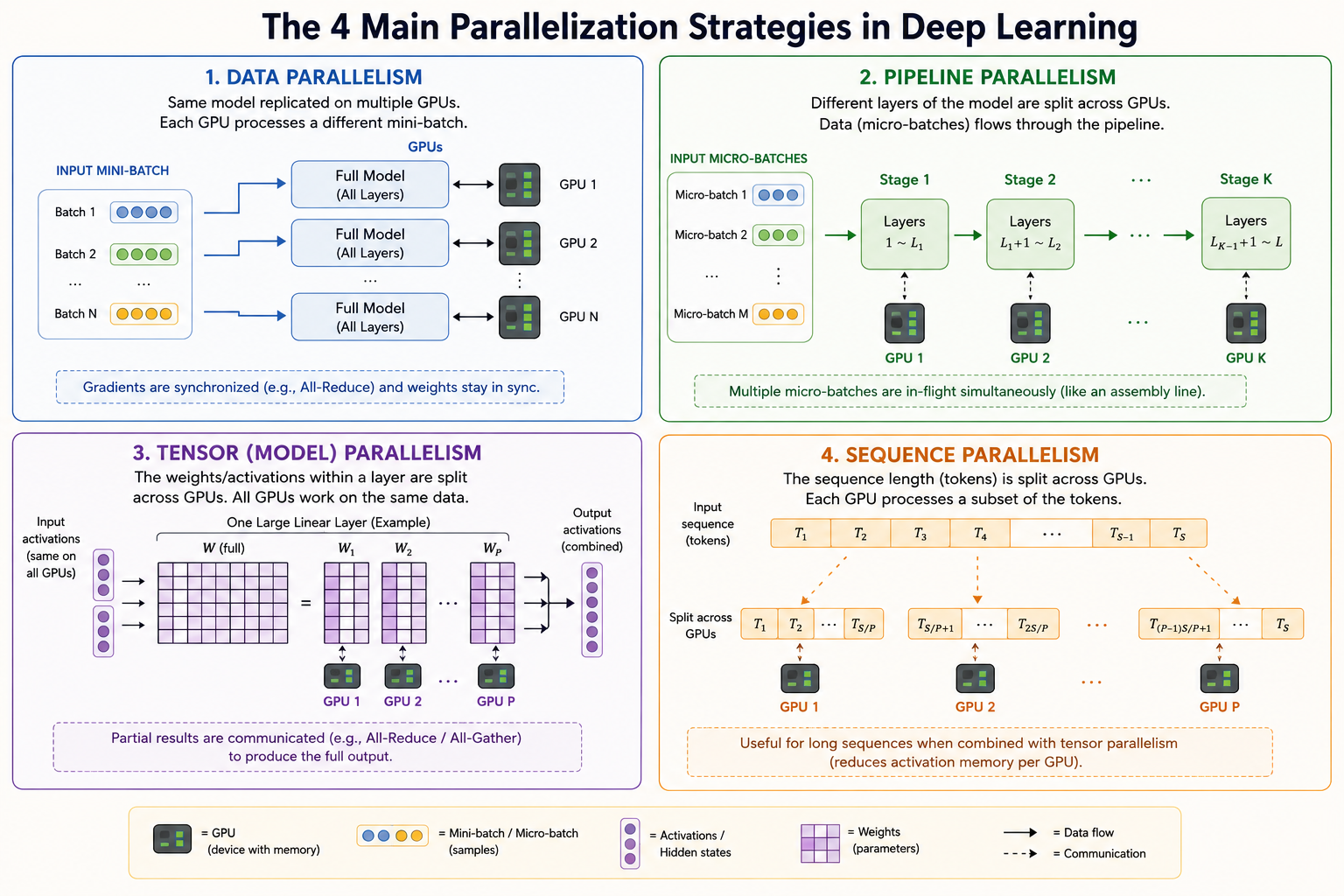
The main techniques split either the data, the model layers, the tensors inside layers, or the sequence dimension.

Parallelization Methods

Data Parallelization

Data parallelism gives every device a copy of the same model, but sends each device a different mini-batch.

Each iteration follows this pattern:

1. **Replicate:**every device starts with the same model weights.
2. **Forward:**each device computes loss on its local mini-batch.
3. **Backward:**each device computes local gradients.
4. **Synchronize:**devices average gradients, usually withAll\-Reduce.
5. **Update:**every device applies the same averaged gradient update.

The model stays replicated, while the data is partitioned.

Pipeline Parallelization

Pipeline parallelism splits model layers into stages. For example, a 100-layer model might assign:

• layers 1-25 to GPU 1
• layers 26-50 to GPU 2
• layers 51-75 to GPU 3
• layers 76-100 to GPU 4

Data flows sequentially through the stages. To reduce idle time, the batch is split into micro-batches so different GPUs can work on different micro-batches at the same time.

Tensor Parallelization

Tensor parallelism partitions the tensors inside a layer. Large matrix multiplications in linear layers and attention blocks are split across GPUs.

A device computes only its local slice of the matrix multiplication. The partial results are then combined with collectives such asAll\-ReduceorAll\-Gather.

Sequence Parallelization

Sequence parallelism partitions the sequence dimension. Each device processes only a subset of tokens.

This helps long-context training because each device stores and computes over fewer tokens. The challenge is that attention, normalization, and softmax often need global sequence information, so devices must exchange partial results.

Data Parallelization

Parameter Server

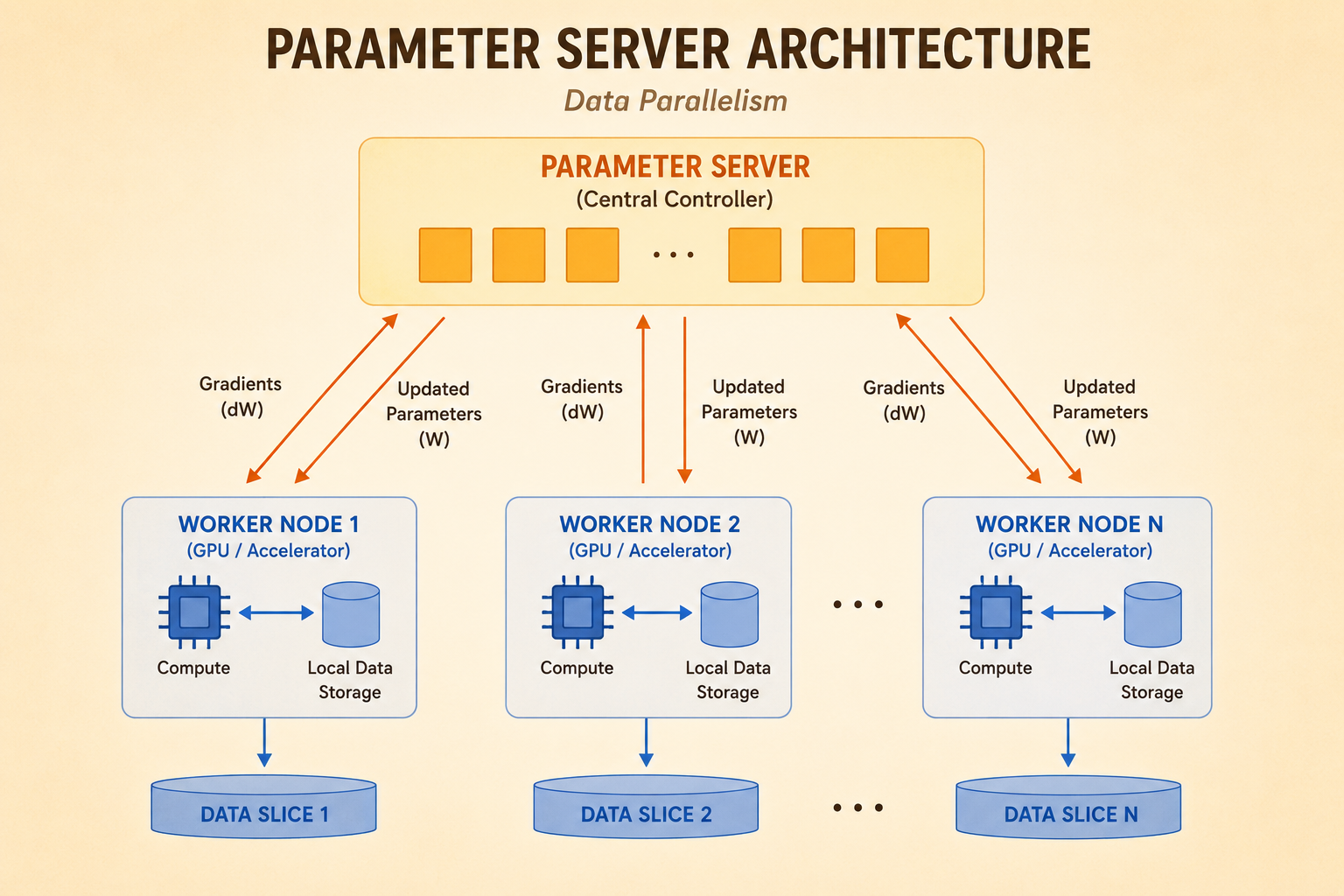
A parameter-server setup separates the global model state from the worker computation.

• **Parameter server:**receives gradients, aggregates them, and sends updated model weights back.
• **Workers:**hold local data shards, compute local gradients, and communicate with the server.
• **Global state:**the parameter server keeps the model consistent across workers.

Single Node vs. Distributed Training

Single-node training has a simple iteration:

\[ \text{sample} \rightarrow \text{compute gradients} \rightarrow \text{update weights} \]

Distributed training adds communication:

\[ \text{pull weights} \rightarrow \text{sample} \rightarrow \text{compute gradients} \rightarrow \text{push gradients} \rightarrow \text{global update} \]

The benefit is parallel compute. The cost is synchronization and communication overhead.

Communication Primitives

Distributed training depends on communication collectives. The model-parallel strategy determines which collective appears on the critical path.

One-to-One

Point-to-point communication sends data from one process to another specific process.

Example:

node 0 -> node 3

Scatter and Gather

Scatteris one-to-many. A source node splits a tensor into chunks and sends one chunk to each worker.

Gatheris many-to-one. Workers send local results back to a source node, which reconstructs the full tensor.

Reduce and Broadcast

Reduceaggregates values from many workers into one result. For example:

\[ [1] + [2] + [3] + [4] = [10] \]

Broadcastsends one tensor from a source node to every other node.

All-Reduce and All-Gather

All-Reducecombines reduce and broadcast. Every worker contributes data, and every worker receives the same aggregated result.

This is the core operation in synchronous data parallel training:

\[ g = \frac{1}{N} \sum_{i=1}^{N} g_i \]

where\(g_i\)is the gradient from worker\(i\).

All-Gathergathers data from all workers and distributes the full concatenated result back to all workers.

MethodTime ComplexityPeak Node BandwidthTotal BandwidthParameter Server\(O(1)\)\(O(N)\)\(O(N)\)All-Reduce: Sequential\(O(N)\)\(O(N)\)\(O(N)\)All-Reduce: Ring\(O(N)\)\(O(1)\)\(O(N)\)All-Reduce: Parallel\(O(1)\)\(O(N)\)\(O(N^2)\)

Recursive All-Reduce

Recursive all-reduce uses a doubling or halving communication pattern.

At each step, nodes exchange with partners at increasing offsets:

1. offset 1
2. offset 2
3. offset 4
4. continue until all nodes have contributed

This reaches global synchronization in:

\[ \log_2(N) \]

communication steps.

ZeRO and FSDP

Memory Usage During Training

Using FP16 weights as a simple example:

• weights: 2 bytes per parameter
• gradients: 2 bytes per parameter
• Adam optimizer states: about 12 bytes per parameter

So the standard replicated memory cost is roughly:

\[ 2 + 2 + 12 = 16 \text{ bytes per parameter} \]

On an 80 GB GPU:

\[ \frac{80\text{ GB}}{16\text{ bytes}} \approx 5.0 \text{ billion parameters} \]

This is far below the scale of large language models, so simply replicating all training states on every GPU does not scale.

ZeRO-1: Shard Optimizer States

ZeRO-1 partitions optimizer states across\(N\)GPUs.

Weights and gradients are still replicated, but each GPU stores only:

\[ \frac{1}{N} \]

of the optimizer states.

Approximate memory per parameter:

\[ 2 + 2 + \frac{12}{N} \]

For\(N=64\):

\[ 2 + 2 + \frac{12}{64} \approx 4.2 \text{ bytes per parameter} \]

This raises the model capacity to roughly 19 billion parameters on 80 GB GPUs.

ZeRO-2: Shard Optimizer States and Gradients

ZeRO-2 additionally shards gradients.

Approximate memory per parameter:

\[ 2 + \frac{2}{N} + \frac{12}{N} \]

For\(N=64\):

\[ 2 + \frac{2}{64} + \frac{12}{64} \approx 2.2 \text{ bytes per parameter} \]

This raises the capacity to roughly 36 billion parameters on 80 GB GPUs.

ZeRO-3: Shard Parameters, Gradients, and Optimizer States

ZeRO-3 shards all three major training states:

• parameters
• gradients
• optimizer states

Approximate memory per parameter:

\[ \frac{2}{N} + \frac{2}{N} + \frac{12}{N} = \frac{16}{N} \]

For\(N=64\):

\[ \frac{16}{64} = 0.25 \text{ bytes per parameter} \]

With 80 GB GPUs, this makes hundreds-of-billions-parameter training feasible.

In PyTorch, ZeRO-3-style sharding is implemented throughFully Sharded Data Parallel, orFSDP.

Pipeline Parallelism

Naive Pipeline Parallelism

Naive pipeline parallelism splits model layers across GPUs, but each stage waits for the previous stage before it can run.

This creates thepipeline bubble:

• early GPUs become idle after sending activations forward
• later GPUs wait before they receive work
• the hardware is underutilized

GPipe

GPipe reduces the bubble by splitting a large batch into micro-batches.

For example:

\[ [16, 10, 512] \rightarrow 4 \times [4, 10, 512] \]

Once GPU 0 finishes the first micro-batch, it sends it to GPU 1 and immediately starts the next micro-batch. Multiple stages can then work concurrently on different micro-batches.

The goal is to keep all pipeline stages busy for most of the iteration.

Tensor Parallelism

Tensor parallelism slices large weight tensors so a single layer operation can be distributed across devices.

FFN Layer

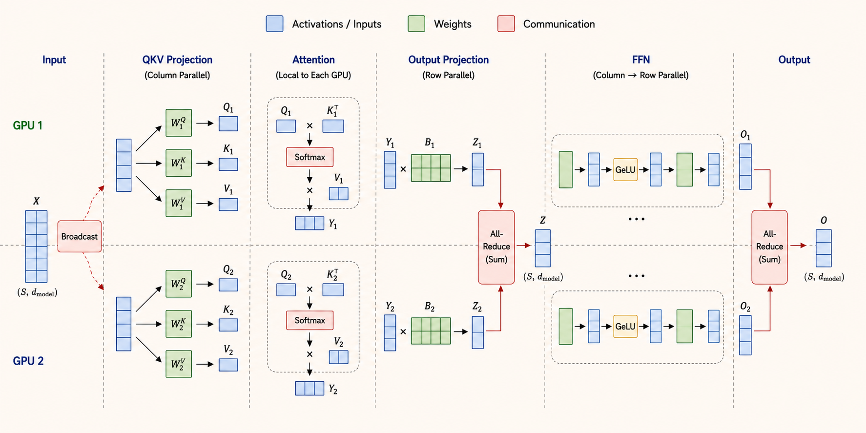
A Transformer feed-forward network often has the form:

\[ X \rightarrow A \rightarrow \operatorname{GeLU} \rightarrow B \rightarrow Z \]

The common strategy is:

1. Split\(A\)column-wise.
2. Apply GeLU independently on each local activation slice.
3. Split\(B\)row-wise.
4. UseAll\-Reduceat the end to sum partial outputs.

This avoids communication between the two matrix multiplications and pays the communication cost only after the second projection.

QKV Projection

For attention, the query, key, and value projections are often split column-wise.

Each GPU computes only a subset of attention heads:

\[ Q_i,\ K_i,\ V_i \]

The input\(X\)is broadcast to each device, and every device computes its local projection independently.

Attention and Output Projection

After local attention heads are computed, the output projection is usually row-parallel.

Each device multiplies its local activation slice by its local row shard of the output matrix. The partial outputs are then summed withAll\-Reduce:

\[ Z = \sum_i Z_i \]

Sequence Parallelism

Repartition Data in Attention Layers

Sequence parallelism splits tokens across GPUs. This increases the maximum sequence length that can be processed because each GPU owns only a partition of the full context.

The scaling rule is:

\[ \#\text{GPUs} = \#\text{sequence partitions} = \#\text{head partitions} \]

Attention still needs global information, so sequence-parallel attention often requiresAll\-to\-Allcommunication.

Ring Attention

Ring attention distributes keys and values across GPUs.

Each GPU holds:

• local queries\(Q\)
• one shard of keys\(K\)
• one shard of values\(V\)

GPUs pass\(K\)and\(V\)blocks around a ring. While a GPU receives a new block, it computes attention scores for its local queries against that block.

The key idea is overlapping:

\[ \text{communication} \quad \text{with} \quad \text{attention computation} \]

This makes long-context attention more scalable than gathering all keys and values onto every device.

Source: Efficient AI, Lecture 19: Distributed Training Part 1.