The Curse of Depth in Large Language Models

# The Curse of Depth in Large Language Models
Source: [https://arxiv.org/html/2502.05795](https://arxiv.org/html/2502.05795)
Wenfang Sun∗1, Xinyuan Song∗2, Pengxiang Li∗3, Lu Yin4, Yefeng Zheng1, Shiwei Liu†5 1Westlake University, China 2Emory University, USA 3Dalian University of Technology, China 4University of Surrey, UK 5University of Oxford, UK

###### Abstract

In this paper, we introducethe Curse of Depth, a concept that highlights, explains, and addresses the recent observation in modern Large Language Models \(LLMs\) where nearly half of the layers are less effective than expected\. We first confirm the wide existence of this phenomenon across the most popular families of LLMs such as Llama, Mistral, DeepSeek, and Qwen\. Our analysis, theoretically and empirically, identifies that the underlying reason for the ineffectiveness of deep layers in LLMs is the widespread usage of Pre\-Layer Normalization \(Pre\-LN\)\. While Pre\-LN stabilizes the training of Transformer LLMs, its output variance exponentially grows with the model depth, which undesirably causes the derivative of the deep Transformer blocks to be an identity matrix, and therefore barely contributes to the training\. To resolve this training pitfall, we proposeLayerNorm Scaling \(LNS\), which scales the variance of output of the layer normalization inversely by the square root of its depth\.111We found that combining LNS with Scaled Initialization\(Groeneveldet al\.,[2024](https://arxiv.org/html/2502.05795v5#bib.bib78); Radfordet al\.,[2019](https://arxiv.org/html/2502.05795v5#bib.bib71); Shoeybiet al\.,[2020](https://arxiv.org/html/2502.05795v5#bib.bib48)\)diminishes the effectiveness of LNS\. Therefore, we recommend removing the latter when applying LNS\.This simple modification mitigates the output variance explosion of deeper Transformer layers, improving their contribution\. Across a wide range of model sizes \(130M to 7B\), our experiments show that LNS consistently outperforms previous normalization and scaling techniques in enhancing LLM pre\-training performance\. Moreover, this improvement seamlessly carries over to supervised fine\-tuning\. All these gains can be attributed to the fact that LayerNorm Scaling enables deeper layers to contribute more effectively during training\. Our code is available at[LayerNorm\-Scaling](https://github.com/lmsdss/LayerNorm-Scaling)\.

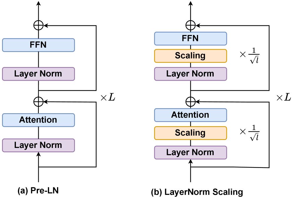
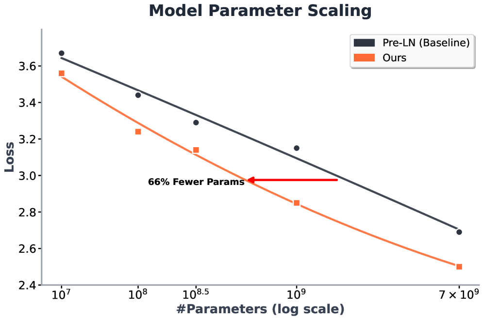
\*\*footnotetext:Equal contribution\. Accepted at NeurIPS 2025\.††footnotetext:Correspondence to: Shiwei Liu, shiwei\.liu@maths\.ox\.ac\.uk\.![Refer to caption](https://arxiv.org/html/2502.05795v5/x1.png)

![Refer to caption](https://arxiv.org/html/2502.05795v5/x2.png)

Figure 1:Left:Schematic diagrams of \(a\) Pre\-LN and \(b\) LayerNorm Scaling\. LayerNorm Scaling applies a scaling factor inversely proportional to the square root of the layer indexℓ\\ell, preventing excessive variance growth\.Right: Language modeling loss of scaling up parameter count up to 7B\. All models are trained for 20B tokens using OLMo\(Groeneveldet al\.,[2024](https://arxiv.org/html/2502.05795v5#bib.bib78)\)\.###### Contents

1. [1Introduction](https://arxiv.org/html/2502.05795v5#S1)
2. [2Empirical Evidence of the Curse of Depth](https://arxiv.org/html/2502.05795v5#S2)1. [2\.1Open\-weight Large\-scale LLMs](https://arxiv.org/html/2502.05795v5#S2.SS1) 2. [2\.2In\-house Small\-scale LLaMa\-130M](https://arxiv.org/html/2502.05795v5#S2.SS2)
3. [3Analysis of the Curse of Depth](https://arxiv.org/html/2502.05795v5#S3)1. [3\.1Pre\-LN Transformers](https://arxiv.org/html/2502.05795v5#S3.SS1)
4. [4LayerNorm Scaling \(LNS\)](https://arxiv.org/html/2502.05795v5#S4)1. [4\.1Theoretical Analysis of LayerNorm Scaling](https://arxiv.org/html/2502.05795v5#S4.SS1)
5. [5Experiments](https://arxiv.org/html/2502.05795v5#S5)1. [5\.1LLM Pre\-training](https://arxiv.org/html/2502.05795v5#S5.SS1) 2. [5\.2Supervised Fine\-tuning](https://arxiv.org/html/2502.05795v5#S5.SS2) 3. [5\.3Scaling Up Training](https://arxiv.org/html/2502.05795v5#S5.SS3)1. [5\.3\.1OLMo](https://arxiv.org/html/2502.05795v5#S5.SS3.SSS1) 2. [5\.3\.2Qwen2\.5](https://arxiv.org/html/2502.05795v5#S5.SS3.SSS2) 4. [5\.4LNS Effectively Scales Down Output Variance](https://arxiv.org/html/2502.05795v5#S5.SS4) 5. [5\.5LNS Enhances the Effectiveness of Deep Layers](https://arxiv.org/html/2502.05795v5#S5.SS5) 6. [5\.6LayerNorm Scaling in Vision Transformer](https://arxiv.org/html/2502.05795v5#S5.SS6)
6. [6Ablation Study](https://arxiv.org/html/2502.05795v5#S6)
7. [7Related Work](https://arxiv.org/html/2502.05795v5#S7)
8. [8Conclusion](https://arxiv.org/html/2502.05795v5#S8)
9. [AProofs of the Theorems of curse of depth](https://arxiv.org/html/2502.05795v5#A1)1. [A\.1Proof of Lemma3\.2](https://arxiv.org/html/2502.05795v5#A1.SS1)1. [A\.1\.1Variance of the Attention](https://arxiv.org/html/2502.05795v5#A1.SS1.SSS1) 2. [A\.1\.2Variance of the Feed\-Forward Network](https://arxiv.org/html/2502.05795v5#A1.SS1.SSS2) 2. [A\.2Proof of Theorem3\.3](https://arxiv.org/html/2502.05795v5#A1.SS2)1. [A\.2\.1Proof of Lemma36](https://arxiv.org/html/2502.05795v5#A1.SS2.SSS1) 2. [A\.2\.2Analysis of the Upper Bound](https://arxiv.org/html/2502.05795v5#A1.SS2.SSS2) 3. [A\.3Proof of Lemma4\.1](https://arxiv.org/html/2502.05795v5#A1.SS3) 4. [A\.4Proof of Theorem17](https://arxiv.org/html/2502.05795v5#A1.SS4) 5. [A\.5Proof of theorem4\.3](https://arxiv.org/html/2502.05795v5#A1.SS5)
10. [BVariance Growth in Pre\-LN Training](https://arxiv.org/html/2502.05795v5#A2)
11. [CPerformance Drop of Layer Pruning in Vision–Language Models \(Qwen 2\.5\-VL\)](https://arxiv.org/html/2502.05795v5#A3)
12. [DLimitations](https://arxiv.org/html/2502.05795v5#A4)

## 1Introduction

Recent studies reveal that the deeper layers \(Transformer blocks\) in modern LLMs tend to be less effective than the earlier ones\(Yinet al\.,[2024](https://arxiv.org/html/2502.05795v5#bib.bib60); Gromovet al\.,[2024](https://arxiv.org/html/2502.05795v5#bib.bib52); Menet al\.,[2024](https://arxiv.org/html/2502.05795v5#bib.bib10); Liet al\.,[2024b](https://arxiv.org/html/2502.05795v5#bib.bib76)\)\. On the one hand, this interesting observation provides an effective indicator for LLM compression\. For instance, we can compress deeper layers significantly more\(Yinet al\.,[2024](https://arxiv.org/html/2502.05795v5#bib.bib60); Luet al\.,[2024](https://arxiv.org/html/2502.05795v5#bib.bib50); Dumitruet al\.,[2024](https://arxiv.org/html/2502.05795v5#bib.bib47)\)to achieve high compression ratios\. Even more aggressively, entire deep layers can be pruned completely without compromising performance\(Muralidharanet al\.,[2024](https://arxiv.org/html/2502.05795v5#bib.bib49); Siddiquiet al\.,[2024](https://arxiv.org/html/2502.05795v5#bib.bib46)\)\.

On the other hand, having many layers ineffective is undesirable as modern LLMs are extremely resource\-intensive to train, often requiring thousands of GPUs trained for multiple months, let alone the labor used for data curation and administrationAchiamet al\.\([2023](https://arxiv.org/html/2502.05795v5#bib.bib75)\); Touvronet al\.\([2023](https://arxiv.org/html/2502.05795v5#bib.bib62)\)\. Ideally, we want all layers in a model to be well\-trained, with sufficient diversity in features from layer to layer, to maximize the utility of resources\(Liet al\.,[2024b](https://arxiv.org/html/2502.05795v5#bib.bib76)\)\. The existence of ill\-trained layers suggests that there must be something off with current LLM paradigms\. Addressing such limitations is a pressing need for the community to avoid the waste of valuable resources, as new versions of LLMs are usually trained with their previous computing paradigm which results in ineffective layers\.

To seek the immediate attention of the community, we re\-introduce the concept ofthe Curse of Depth \(CoD\)to systematically present the phenomenon of ineffective deep layers in various LLM families, to identify the underlying reason behind it, and to rectify it by proposing LayerNorm Scaling\. We first statethe Curse of Depthbelow\.

The Curse of Depth\.The Curse of Depthrefers to the observed phenomenon where deeper layers in modern LLMs contribute significantly less \(but not nothing\) to learning and representation compared to earlier layers\. These deeper layers often exhibit remarkable robustness to pruning and perturbations, implying they fail to perform meaningful transformations\. This behavior prevents these layers from effectively contributing to training and representation learning, resulting in resource inefficiency\.

Empirical Evidence of CoD\.To demonstrate that CoD is a common phenomenon across prominent LLM families, we perform layer pruning experiments on Qwen3, LLaMA2, and DeepSeek\. Specifically, we prune one layer at a time, without any fine\-tuning, and directly evaluate the resulting pruned models on the MMLU benchmark\(Hendryckset al\.,[2021](https://arxiv.org/html/2502.05795v5#bib.bib27)\), as shown in Figure[2](https://arxiv.org/html/2502.05795v5#S1.F2)\.Key findings:\(1\) Most models, including the latest Qwen3, exhibit surprising resilience to the removal of deeper layers; \(2\) The number of layers that can be removed without causing significant performance drop increases with model size; \(3\) Representations in deeper layers are significantly more similar to each other than those in earlier layers\.

Identifying the Root Cause of CoD\.We theoretically and empirically identify the root cause of CoD as the use of Pre\-Layer Normalization \(Pre\-LN\)\(Baevski and Auli,[2019](https://arxiv.org/html/2502.05795v5#bib.bib28); Daiet al\.,[2019](https://arxiv.org/html/2502.05795v5#bib.bib33)\), which normalizes layer inputs before applying the main computations, such as attention or feedforward operations, rather than after\. Specifically, while stabilizing training, we observe that the output variance of Pre\-LN accumulates significantly with layer depth as shown in Figure[4](https://arxiv.org/html/2502.05795v5#S2.F4), causing the derivatives of deep Pre\-LN layers to approach an identity matrix\. This behavior prevents these layers from introducing meaningful transformations, leading to diminished representation learning\.

Mitigating CoD through LayerNorm Scaling\.We propose LayerNorm Scaling \(LNS\), which scales the output of Layer Normalization by the square root of the depth1l\\frac\{1\}\{\\sqrt\{l\}\}\. LayerNorm Scaling effectively scales down the output variance across layers of Pre\-LN\. LNS consistently delivers better pre\-training performance than existing normalization and scaling techniques across various model sizes from 130M to 7B\. Unlike previous LayerNorm variants\(Liet al\.,[2024b](https://arxiv.org/html/2502.05795v5#bib.bib76); Liuet al\.,[2020](https://arxiv.org/html/2502.05795v5#bib.bib54)\), LayerNorm Scaling is simple to implement, requires no hyperparameter tuning, and introduces no additional parameters during training\. Furthermore, we show that the model pre\-trained with LayerNorm Scaling achieves better performance on downstream tasks in self\-supervised fine\-tuning, all thanks to the more diverse feature representations learned in deep layers\.

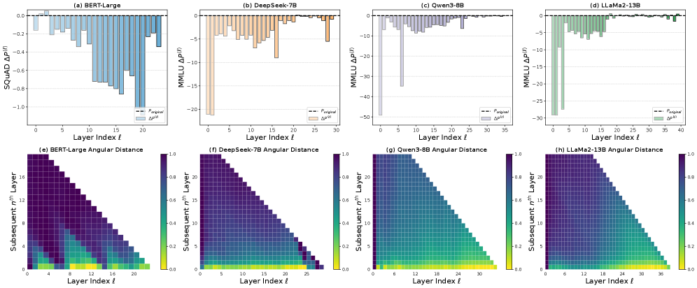![Refer to caption](https://arxiv.org/html/2502.05795v5/x3.png)Figure 2:Results of open\-weight large\-scale LLMs\.Top:Performance drop after removing a single layer without fine\-tuning\.Bottom:Angular distance from the initial layerℓ\\ell\(x\-axis\) and its subsequentnthn^\{\\text\{th\}\}layer \(y\-axis\)\. The results demonstrate that in Pre\-LN LLMs, deeper layers produce highly similar representations to their adjacent layers, and their removal results in minimal performance degradation\. In contrast, Post\-LN models show the opposite trend: deep layers contribute more substantially to model performance\.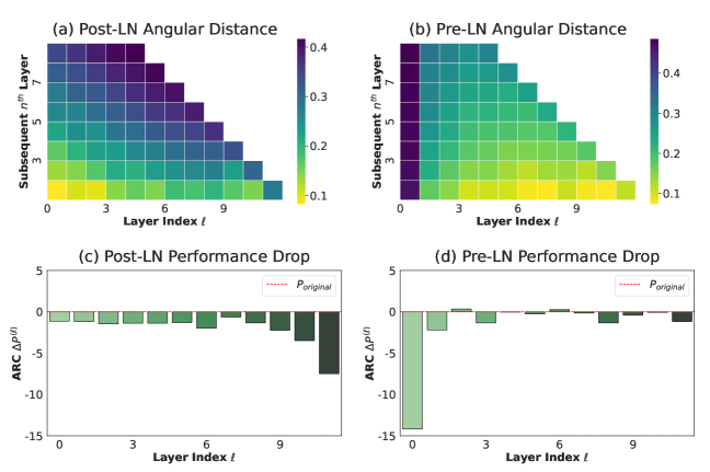![Refer to caption](https://arxiv.org/html/2502.05795v5/x4.png)Figure 3:Results of in\-house small\-scale LLaMa\-130M\.Angular Distance \(a, b\): Each column represents the angular distance from the initial layerℓ\\ell\(x\-axis\) and its subsequentnt​hn^\{th\}layer \(y\-axis\)\. The distance is scaled to the range \[0, 1\], where yellow indicates smaller distances and purple indicates larger distances\.Performance Drop \(c, d\): ARC\-e performance drop of removing each single layer from LLaMa\-130M\.
## 2Empirical Evidence of the Curse of Depth

To empirically analyze the impact of layer normalization on theCurse of Depthin LLMs, we conduct a series of evaluations inspired byLiet al\.\([2024b](https://arxiv.org/html/2502.05795v5#bib.bib76)\), to compare Pre\-LN and Post\-LN models\.

Methodology:We evaluate Pre\-LN and Post\-LN models by assessing the impact of layer pruning at different depths\. Our hypothesis is that Pre\-LN models exhibit diminishing effectiveness in deeper layers, whereas Post\-LN models have less effective early layers\.

### 2\.1Open\-weight Large\-scale LLMs

Models:To verify this, we empirically quantify the contribution of individual layers to overall model performance across a diverse set of LLMs, including Qwen3\(Team,[2025](https://arxiv.org/html/2502.05795v5#bib.bib72)\), LLaMA2\(Touvronet al\.,[2023](https://arxiv.org/html/2502.05795v5#bib.bib62)\), DeepSeek\(Biet al\.,[2024](https://arxiv.org/html/2502.05795v5#bib.bib56)\), and BERT\-Large\(Devlin,[2019](https://arxiv.org/html/2502.05795v5#bib.bib30)\)\. These models were chosen to ensure architectural and application diversity\. BERT\-Large represents a Post\-LN model, whereas the rest are Pre\-LN\-based\. This selection enables a comprehensive evaluation of the effects of layer normalization across varying architectures and model scales\.

Evaluation Metric:To empirically assess the impact of deeper layers in LLMs, we adopt two metrics,Performance DropandAngular Distance, inspired byGromovet al\.\([2024](https://arxiv.org/html/2502.05795v5#bib.bib52)\); Liet al\.\([2024b](https://arxiv.org/html/2502.05795v5#bib.bib76)\)\.

Performance DropΔ​P\(ℓ\)\\Delta P^\{\(\\ell\)\}quantifies the importance of each layer by measuring the performance change after its removal\. A smallerΔ​P\(ℓ\)\\Delta P^\{\(\\ell\)\}indicates that the pruned layer contributes less to the model’s overall performance\. For BERT\-Large, we evaluate using the SQuAD v1\.1 dataset\(Rajpurkar,[2016](https://arxiv.org/html/2502.05795v5#bib.bib26)\), while for other models, we use MMLU\(Hendryckset al\.,[2021](https://arxiv.org/html/2502.05795v5#bib.bib27)\), a standard benchmark for multi\-task language understanding\.

Angular Distanced​\(xℓ,xℓ\+n\)d\(x^\{\\ell\},x^\{\\ell\+n\}\)quantifies the directional change between the input representations at layerℓ\\elland layerℓ\+n\\ell\+non a neutral pre\-training dataset\. Formally, given a tokenTT, letxTℓx\_\{T\}^\{\\ell\}andxTℓ\+nx\_\{T\}^\{\\ell\+n\}denote its input to layersℓ\\ellandℓ\+n\\ell\+n, respectively\. The angular distance is defined as:

d​\(xℓ,xℓ\+n\)=1π​arccos⁡\(xTℓ⋅xTℓ\+n‖xTℓ‖2​‖xTℓ\+n‖2\),d\(x^\{\\ell\},x^\{\\ell\+n\}\)=\\frac\{1\}\{\\pi\}\\arccos\\left\(\\frac\{x\_\{T\}^\{\\ell\}\\cdot x\_\{T\}^\{\\ell\+n\}\}\{\\\|x\_\{T\}^\{\\ell\}\\\|\_\{2\}\\\|x\_\{T\}^\{\\ell\+n\}\\\|\_\{2\}\}\\right\),\(1\)where∥⋅∥2\\\|\\cdot\\\|\_\{2\}denotes theL2L^\{2\}\-norm\. To reduce variance, we report the average distance over 256K tokens sampled from the C4 dataset\. Smaller values ofd​\(xℓ,xℓ\+n\)d\(x^\{\\ell\},x^\{\\ell\+n\}\)indicate higher similarity between the two representations, suggesting limited transformation\. Such layers can be considered redundant, as their removal minimally impacts the model’s internal representations\. Ideally, each layer should introduce meaningful representational shifts to fully leverage the model’s capacity\(Yanget al\.,[2023](https://arxiv.org/html/2502.05795v5#bib.bib18); Gromovet al\.,[2024](https://arxiv.org/html/2502.05795v5#bib.bib52)\)\.

Experimental Results:\(1\) Pruning deep layers in Pre\-LN LLMs leads to negligible, and sometimes even positive, changes in performance, as shown in Figure[2](https://arxiv.org/html/2502.05795v5#S1.F2)\-Top\. Specifically, Figure[2](https://arxiv.org/html/2502.05795v5#S1.F2)\(b\)–\(d\) reveals that a wide range of deeper layers—particularly beyond the 18th—can be pruned with minimal impact on performance\. This indicates that deep layers in Pre\-LN architectures contribute little to the model’s overall effectiveness\. In contrast, Figure[2](https://arxiv.org/html/2502.05795v5#S1.F2)\(a\) shows that pruning deep layers in BERT\-Large \(a Post\-LN model\) leads to a substantial drop in accuracy, while pruning early layers has a relatively minor effect\. \(2\) Pre\-LN models exhibit decreasing angular distance in deeper layers, indicating highly similar representations, as shown in Figure[2](https://arxiv.org/html/2502.05795v5#S1.F2)\-Bottom\. For instance, the angular distance in DeepSeek\-7B falls below 0\.2 after the 18th layer\. Qwen3\-8B demonstrates a higher similarity, with nearly half of its layers exhibiting distances below 0\.2 from their preceding layers\. In LLaMA2\-13B, the angular distance approaches zero across the final one\-third of the network\. These similar representations align with the pruning results in Figures[2](https://arxiv.org/html/2502.05795v5#S1.F2)\(b\)–\(d\), where pruning later layers has little effect, while pruning early layers significantly degrades performance\.

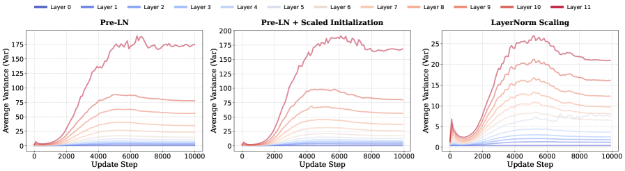![Refer to caption](https://arxiv.org/html/2502.05795v5/x5.png)Figure 4:Layerwise output variance\.This figure compares the output variance across various layers for different setups: \(1\) Pre\-LN; \(2\) Pre\-LN with Scaled Initialization\(Shoeybiet al\.,[2020](https://arxiv.org/html/2502.05795v5#bib.bib48); Radfordet al\.,[2019](https://arxiv.org/html/2502.05795v5#bib.bib71)\); and \(3\) LayerNorm Scaling\. The experiments are conducted on the LLaM\-130M model trained for 10,000 steps\. The proposed LayerNorm Scaling effectively controls the variance across layers\.
### 2\.2In\-house Small\-scale LLaMa\-130M

To eliminate the influence of other confounding variables, we train two LLaMA\-130M models from scratch that differ only in their Layer Normalization, thereby clearly distinguishing Post\-LN from Pre\-LN, followingLiet al\.\([2024b](https://arxiv.org/html/2502.05795v5#bib.bib76)\)\. The results are illustrated in Figure[3](https://arxiv.org/html/2502.05795v5#S1.F3)\.

In Post\-LN models, early layers exhibit high similarity \(low angular distance, Figure[3](https://arxiv.org/html/2502.05795v5#S1.F3)\-a\) and their removal causes minimal performance loss \(Figure[3](https://arxiv.org/html/2502.05795v5#S1.F3)\-c\), while deeper layers become more distinct and critical\. Conversely, Pre\-LN LLaMa\-130M demonstrates a gradual decrease in angular distance with depth, resulting in highly similar deep layers \(Figure[3](https://arxiv.org/html/2502.05795v5#S1.F3)\-b\)\. Removing most layers after the first in Pre\-LN causes negligible performance loss \(Figure[3](https://arxiv.org/html/2502.05795v5#S1.F3)\-d\), indicating their limited contribution\. These consistent findings, observed in both open\-weight and in\-house LLMs, lead to the conclusion that the widespread use of Pre\-LN is the root cause of the ineffectiveness of deep layers in LLMs\.

## 3Analysis of the Curse of Depth

Preliminaries\.This paper primarily focuses on Pre\-LN Transformer\(Baevski and Auli,[2019](https://arxiv.org/html/2502.05795v5#bib.bib28); Daiet al\.,[2019](https://arxiv.org/html/2502.05795v5#bib.bib33)\)\. Letxℓ∈ℝdx\_\{\\ell\}\\in\\mathbb\{R\}^\{d\}be the input vector at theℓ\\ell\-th layer of Transformer, wheredddenotes the feature dimension of each layer\. For simplicity, we assume all layers to have the same dimensiondd\. The layer outputyyis calculated as follows:

y=xℓ\+1=xℓ′\+FFN​\(LN​\(xℓ′\)\),y=x\_\{\\ell\+1\}=x^\{\\prime\}\_\{\\ell\}\+\\mathrm\{FFN\}\(\\mathrm\{LN\}\(x^\{\\prime\}\_\{\\ell\}\)\),\(2\)xℓ′=xℓ\+Attn​\(LN​\(xℓ\)\),x^\{\\prime\}\_\{\\ell\}=x\_\{\\ell\}\+\\mathrm\{Attn\}\(\\mathrm\{LN\}\(x\_\{\\ell\}\)\),\(3\)where LN denotes the layer normalization function\. In addition, the feed\-forward network \(FFN\) and the multi\-head self\-attention \(Attn\) sub\-layers are defined as follows:

FFN​\(x\)\\displaystyle\\mathrm\{FFN\}\(x\)=W2​ℱ​\(W1​x\),\\displaystyle=W\_\{2\}\\mathcal\{F\}\(W\_\{1\}x\),\(4\)Attn​\(x\)\\displaystyle\\mathrm\{Attn\}\(x\)=WO​\(concat​\(head1​\(x\),…,headh​\(x\)\)\),\\displaystyle=W\_\{O\}\(\\mathrm\{concat\}\(\\mathrm\{head\}\_\{1\}\(x\),\\dots,\\mathrm\{head\}\_\{h\}\(x\)\)\),headi​\(x\)\\displaystyle\\mathrm\{head\}\_\{i\}\(x\)=softmax​\(\(WQ​i​x\)⊤​\(WK​i​X\)dhead\)​\(WV​i​X\)⊤,\\displaystyle=\\mathrm\{softmax\}\\left\(\\frac\{\(W\_\{Qi\}x\)^\{\\top\}\(W\_\{Ki\}X\)\}\{\\sqrt\{d\_\{\\mathrm\{head\}\}\}\}\\right\)\(W\_\{Vi\}X\)^\{\\top\},whereℱ\\mathcal\{F\}is an activation function,concat\\mathrm\{concat\}concatenates input vectors,softmax\\mathrm\{softmax\}applies the softmax function, andW1∈ℝdffn×dW\_\{1\}\\in\\mathbb\{R\}^\{d\_\{\\mathrm\{ffn\}\}\\times d\},W2∈ℝd×dffnW\_\{2\}\\in\\mathbb\{R\}^\{d\\times d\_\{\\mathrm\{ffn\}\}\},WQ​i∈ℝdhead×dW\_\{Qi\}\\in\\mathbb\{R\}^\{d\_\{\\mathrm\{head\}\}\\times d\},WK​i∈ℝdhead×dW\_\{Ki\}\\in\\mathbb\{R\}^\{d\_\{\\mathrm\{head\}\}\\times d\},WV​i∈ℝdhead×dW\_\{Vi\}\\in\\mathbb\{R\}^\{d\_\{\\mathrm\{head\}\}\\times d\}, andWO∈ℝd×dW\_\{O\}\\in\\mathbb\{R\}^\{d\\times d\}are parameter matrices, anddFFNd\_\{\\mathrm\{FFN\}\}anddheadd\_\{\\mathrm\{head\}\}are the internal dimensions of FFN and multi\-head self\-attention sub\-layers, respectively\.X∈ℝd×sX\\in\\mathbb\{R\}^\{d\\times s\}, wheressis the input sequence length\.

The derivatives of Pre\-Ln Transformers are:

∂Pre\-LN​\(x\)∂x=I\+∂f​\(LN​\(x\)\)∂LN​\(x\)​∂LN​\(x\)∂x,\\frac\{\\partial\\text\{Pre\-LN\}\(x\)\}\{\\partial x\}=I\+\\frac\{\\partial f\(\\text\{LN\}\(x\)\)\}\{\\partial\\text\{LN\}\(x\)\}\\frac\{\\partial\\text\{LN\}\(x\)\}\{\\partial x\},\(5\)whereffhere represents either the multi\-head attention function or the FFN function\. If the term∂f​\(LN​\(x\)\)∂LN​\(x\)​∂LN​\(x\)∂x\\frac\{\\partial f\(\\text\{LN\}\(x\)\)\}\{\\partial\\text\{LN\}\(x\)\}\\frac\{\\partial\\text\{LN\}\(x\)\}\{\\partial x\}becomes too small, the Pre\-LN layer∂Pre\-LN​\(x\)∂x\\frac\{\\partial\\text\{Pre\-LN\}\(x\)\}\{\\partial x\}behaves like an identity map\. Our main objective is to prevent identity map behavior for very deep Transformer networks\. The first step in this process is to compute the varianceσxℓ2\\sigma^\{2\}\_\{x\_\{\\ell\}\}of vectorxℓx\_\{\\ell\}\.

### 3\.1Pre\-LN Transformers

###### Assumption 3\.1\.

Letxℓx\_\{\\ell\}andxℓ′x^\{\\prime\}\_\{\\ell\}denote the input and intermediate vectors of theℓ\\ell\-th layer\. Moreover, letWℓW\_\{\\ell\}denote the model parameter matrix at theℓ\\ell\-th layer\. We assume that, for all layers,xℓx\_\{\\ell\},xℓ′x^\{\\prime\}\_\{\\ell\}, andWℓW\_\{\\ell\}follow normal and independent distributions with meanμ=0\\mu=0\.

###### Lemma 3\.2\.

Letσxℓ′2\\sigma^\{2\}\_\{x^\{\\prime\}\_\{\\ell\}\}andσxℓ2\\sigma^\{2\}\_\{x\_\{\\ell\}\}denote the variances ofxℓ′x^\{\\prime\}\_\{\\ell\}andxℓx\_\{\\ell\}, respectively\. These two variances exhibit the same overall growth trend, which is:

σxℓ2=σx12​Θ​\(∏k=1ℓ−1\(1\+1σxk\)\),\\sigma^\{2\}\_\{x\_\{\\ell\}\}=\\sigma\_\{x\_\{1\}\}^\{2\}\\Theta\\Bigl\(\\prod\_\{k=1\}^\{\\ell\-1\}\\left\(1\+\\frac\{1\}\{\\sigma\_\{x\_\{k\}\}\}\\right\)\\Bigr\),\(6\)where the growth ofσxℓ2\\sigma^\{2\}\_\{x\_\{\\ell\}\}is sub\-exponential, as shown by the following bounds:

Θ​\(L\)≤σxL2≤Θ​\(exp⁡\(L\)\)\.\\Theta\(L\)\\leq\\sigma^\{2\}\_\{x\_\{L\}\}\\leq\\Theta\(\\exp\(L\)\)\.\(7\)

Here, the notationΘ\\Thetameans: iff​\(x\)∈Θ​\(g​\(x\)\)f\(x\)\\in\\Theta\\bigl\(g\(x\)\\bigr\), then there exist constantsC1,C2C\_\{1\},C\_\{2\}such thatC1​\|g​\(x\)\|≤\|f​\(x\)\|≤C2​\|g​\(x\)\|C\_\{1\}\|g\(x\)\|\\leq\|f\(x\)\|\\leq C\_\{2\}\|g\(x\)\|asx→∞x\\to\\infty\. The lower boundΘ​\(L\)≤σxℓ2\\Theta\(L\)\\leq\\sigma^\{2\}\_\{x\_\{\\ell\}\}indicates thatσxℓ2\\sigma^\{2\}\_\{x\_\{\\ell\}\}grows at least linearly, while the upper boundσxℓ2≤Θ​\(exp⁡\(L\)\)\\sigma^\{2\}\_\{x\_\{\\ell\}\}\\leq\\Theta\(\\exp\(L\)\)implies that its growth does not exceed an exponential function ofLL\.

Based on Assumption[3\.1](https://arxiv.org/html/2502.05795v5#S3.Thmtheorem1)and the work ofTakaseet al\.\([2023b](https://arxiv.org/html/2502.05795v5#bib.bib38)\), we obtain the following:

###### Theorem 3\.3\.

For a Pre\-LN Transformer withLLlayers, using Equations \([2](https://arxiv.org/html/2502.05795v5#S3.E2)\) and \([3](https://arxiv.org/html/2502.05795v5#S3.E3)\), the partial derivative∂yL∂x1\\frac\{\\partial y\_\{L\}\}\{\\partial x\_\{1\}\}can be written as:

∂yL∂x1=∏ℓ=1L−1\(∂yℓ∂xℓ′⋅∂xℓ′∂xℓ\)\.\\frac\{\\partial y\_\{L\}\}\{\\partial x\_\{1\}\}=\\prod\_\{\\ell=1\}^\{L\-1\}\\left\(\\frac\{\\partial y\_\{\\ell\}\}\{\\partial x^\{\\prime\}\_\{\\ell\}\}\\cdot\\frac\{\\partial x^\{\\prime\}\_\{\\ell\}\}\{\\partial x\_\{\\ell\}\}\\right\)\.\(8\)
The Euclidean norm of∂yL∂x1\\frac\{\\partial y\_\{L\}\}\{\\partial x\_\{1\}\}is given by:

‖∂yL∂x1‖2≤∏l=1L−1\(1\+1σxℓ​A\+1σxℓ2​B\),\\left\\\|\\frac\{\\partial y\_\{L\}\}\{\\partial x\_\{1\}\}\\right\\\|\_\{2\}\\leq\\prod\_\{l=1\}^\{L\-1\}\\left\(1\+\\frac\{1\}\{\\sigma\_\{x\_\{\\ell\}\}\}A\+\\frac\{1\}\{\\sigma\_\{x\_\{\\ell\}\}^\{2\}\}B\\right\),\(9\)whereAAandBBare constants for the Transformer network\. Then the upper bound for this norm is given as follows: whenσxℓ2\\sigma^\{2\}\_\{x\_\{\\ell\}\}grows exponentially, \(i\.e\., at its upper bound\), we have:

σxℓ2∼exp⁡\(ℓ\),‖∂yL∂x1‖2≤M,\\sigma^\{2\}\_\{x\_\{\\ell\}\}\\sim\\exp\(\\ell\),\\quad\\left\\\|\\frac\{\\partial y\_\{L\}\}\{\\partial x\_\{1\}\}\\right\\\|\_\{2\}\\leq M,\(10\)where the gradient norm converges to a constantMM\. Conversely, whenσxℓ2\\sigma^\{2\}\_\{x\_\{\\ell\}\}grows linearly \(i\.e\., at its lower bound\), we have

σxℓ2∼ℓ,‖∂yL∂x1‖2≤Θ​\(L\),\\sigma^\{2\}\_\{x\_\{\\ell\}\}\\sim\\ell,\\quad\\left\\\|\\frac\{\\partial y\_\{L\}\}\{\\partial x\_\{1\}\}\\right\\\|\_\{2\}\\leq\\Theta\(L\),\(11\)which means that the gradient norm grows linearly inLL\.

The detailed description ofAAandBB, as well as the complete proof, are provided in Appendix[A\.2](https://arxiv.org/html/2502.05795v5#A1.SS2)\. From Theorem[3\.3](https://arxiv.org/html/2502.05795v5#S3.Thmtheorem3), we observe that when the variance grows exponentially, as the number of layersL→∞L\\to\\infty, the norm‖∂yL∂x1‖2\\left\\\|\\frac\{\\partial y\_\{L\}\}\{\\partial x\_\{1\}\}\\right\\\|\_\{2\}is bounded above by a fixed constantMM\. This result implies that even an infinitely deep Transformer remains stable, and by the Weierstrass Theorem, the network is guaranteed to converge\. Consequently, this implies that for very largeLL, deeper layers behave nearly as anidentity mapfromxℓx\_\{\\ell\}toyℓy\_\{\\ell\}, thereby limiting the model’s expressivity and hindering its ability to learn meaningful transformations\. This phenomenon is empirically illustrated in Figure[5](https://arxiv.org/html/2502.05795v5#S3.F5), where we visualize the Jacobian of the pre\-LN residual blocks across depth in a pre\-trained LLaMA2\-7B model, revealing a clear collapse toward identity mappings in deeper layers\. This outcome is undesirable, therefore, we would instead prefer the variance to increase more gradually—e\.g\., linearly—so that‖∂yL∂x1‖2\\left\\\|\\frac\{\\partial y\_\{L\}\}\{\\partial x\_\{1\}\}\\right\\\|\_\{2\}exhibits linear growth\. This observation highlights the necessity of appropriate variance control mechanisms, such as scaling strategies, to prevent excessive identity mappings and enhance network depth utilization\.

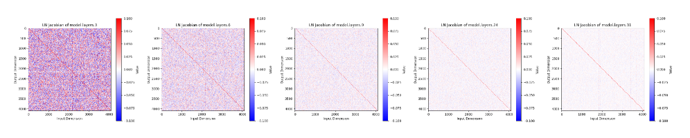![Refer to caption](https://arxiv.org/html/2502.05795v5/x6.png)Figure 5:Visualization of the Jacobian matrices of pre\-LN residual blocks across different layers of a pre\-trained LLaMA2\-7B model\. Each heatmap shows the token\-averaged Jacobian at a specific layer\. As depth increases, the Jacobians exhibit a pronounced diagonal dominance with vanishing off\-diagonal entries, indicating that deep LayerNorm blocks increasingly approximate identity mappings\.

## 4LayerNorm Scaling \(LNS\)

To mitigate the abovementioned issue, we propose LayerNorm Scaling, a simple yet effective normalization strategy\. The core idea of LayerNorm Scaling is to control the exponential growth of output variance in Pre\-LN by scaling the normalized outputs according to layer depth\. Specifically, we apply a scaling factor inversely proportional to the square root of the layer index to scale down the output of LN layers, enhancing the contribution of deeper Transformer layers during training\. LayerNorm Scaling is illustrated in Figure[1](https://arxiv.org/html/2502.05795v5#S0.F1)\.

Formally, for a Transformer model withLLlayers, the output of Layer Normalization in each layerℓ\\ellis scaled by a factor of1ℓ\\frac\{1\}\{\\sqrt\{\\ell\}\}\. Let𝐡\(ℓ\)\\mathbf\{h\}^\{\(\\ell\)\}denote the input to Layer Normalization at layerℓ\\ell\. The modified output is computed as:

𝐡\(ℓ\)=LayerNorm​\(𝐡\(ℓ\)\)×1ℓ,\\mathbf\{h\}^\{\(\\ell\)\}=\\text\{LayerNorm\}\(\\mathbf\{h\}^\{\(\\ell\)\}\)\\times\\frac\{1\}\{\\sqrt\{\\ell\}\},\(12\)whereℓ∈\{1,2,…,L\}\\ell\\in\\\{1,2,\\dots,L\\\}\. This scaling prevents excessive variance growth with depth, addressing a key limitation of Pre\-LN\. Unlike Mix\-LN, which stabilizes gradients in deeper layers but suffers from training instability caused by Post\-LN\(Nguyen and Salazar,[2019](https://arxiv.org/html/2502.05795v5#bib.bib34); Wanget al\.,[2024](https://arxiv.org/html/2502.05795v5#bib.bib59)\), LayerNorm Scaling preserves the stability advantages of Pre\-LN while enhancing the contribution of deeper layers to representation learning\. Applying LayerNorm Scaling leads to a notable reduction of layerwise output variance as shown in Figure[4](https://arxiv.org/html/2502.05795v5#S2.F4), resulting in a lower training loss\. Moreover, compared with previous LayerNorm variants\(Liet al\.,[2024b](https://arxiv.org/html/2502.05795v5#bib.bib76); Liuet al\.,[2020](https://arxiv.org/html/2502.05795v5#bib.bib54)\), LayerNorm Scaling is hyperparameter\-free, easy to implement, and does not introduce additional learnable parameters, making it computationally efficient and readily applicable to existing Transformer architectures\.

### 4\.1Theoretical Analysis of LayerNorm Scaling

###### Lemma 4\.1\.

After applying our scaling method, the variances ofxℓ′x^\{\\prime\}\_\{\\ell\}andxℓx\_\{\\ell\}, denoted asσxℓ′2\\sigma^\{2\}\_\{x^\{\\prime\}\_\{\\ell\}\}andσxℓ2\\sigma^\{2\}\_\{x\_\{\\ell\}\}, respectively, exhibit the same growth trend, which is:

σxℓ2=σx12​Θ​\(∏k=1ℓ−1\(1\+1k​σxk\)\),\\displaystyle\\sigma^\{2\}\_\{x\_\{\\ell\}\}=\\sigma\_\{x\_\{1\}\}^\{2\}\\Theta\\Big\(\\prod^\{\\ell\-1\}\_\{k=1\}\\Big\(1\+\\frac\{1\}\{\\sqrt\{k\}\\sigma\_\{x\_\{k\}\}\}\\Big\)\\Big\),\(13\)with the following growth rate bounds:

Θ​\(L\)≤σxL2≤Θ​\(L\(2−ϵ\)\)\.\\Theta\(L\)\\leq\\sigma^\{2\}\_\{x\_\{L\}\}\\leq\\Theta\(L^\{\(2\-\\epsilon\)\}\)\.\(14\)whereϵ\\epsilonis a small number with1/2≤ϵ<11/2\\leq\\epsilon<1\.

From Lemma[4\.1](https://arxiv.org/html/2502.05795v5#S4.Thmtheorem1), we can conclude that our scaling method effectively slows the growth of the variance upper bound, reducing it from exponential to polynomial growth\. Specifically, it limits the upper bound to a quadratic rate instead of an exponential one\. Based on Theorem[3\.3](https://arxiv.org/html/2502.05795v5#S3.Thmtheorem3), after scaling, we obtain the following:

###### Theorem 4\.2\.

For the scaled Pre\-LN Transformers, the Euclidean norm of∂yL∂x1\\frac\{\\partial y\_\{L\}\}\{\\partial x\_\{1\}\}is given by:

‖∂yL∂x1‖2≤∏ℓ=1L−1\(1\+1ℓ​σxℓ​A\+1ℓ2​σxℓ2​B\),\\left\\\|\\frac\{\\partial y\_\{L\}\}\{\\partial x\_\{1\}\}\\right\\\|\_\{2\}\\leq\\prod\_\{\\ell=1\}^\{L\-1\}\\left\(1\+\\frac\{1\}\{\\ell\\sigma\_\{x\_\{\\ell\}\}\}A\+\\frac\{1\}\{\\ell^\{2\}\\sigma\_\{x\_\{\\ell\}\}^\{2\}\}B\\right\),\(15\)whereAAandBBare dependent on the scaled neural network parameters\. Then the upper bound for the norm is given as follows: whenσxℓ2\\sigma^\{2\}\_\{x\_\{\\ell\}\}grows atℓ\(2−ϵ\)\\ell^\{\(2\-\\epsilon\)\}, \(i\.e\., at its upper bound\), we obtain:

σxℓ2∼ℓ\(2−ϵ\),‖∂yL∂x1‖2≤ω​\(1\),\\sigma^\{2\}\_\{x\_\{\\ell\}\}\\sim\\ell^\{\(2\-\\epsilon\)\},\\quad\\left\\\|\\frac\{\\partial y\_\{L\}\}\{\\partial x\_\{1\}\}\\right\\\|\_\{2\}\\leq\\omega\(1\),\(16\)whereω\\omegadenotes that iff​\(x\)=ω​\(g​\(x\)\)f\(x\)=\\omega\(g\(x\)\), thenlimx→∞f​\(x\)g​\(x\)=∞\\lim\_\{x\\rightarrow\\infty\}\\frac\{f\(x\)\}\{g\(x\)\}=\\infty\. Meanwhile, whenσxℓ2\\sigma^\{2\}\_\{x\_\{\\ell\}\}grows linearly \(i\.e\., at its lower bound\), we obtain:

σxℓ2∼ℓ,‖∂yL∂x1‖2≤Θ​\(L\)\.\\sigma^\{2\}\_\{x\_\{\\ell\}\}\\sim\\ell,\\quad\\left\\\|\\frac\{\\partial y\_\{L\}\}\{\\partial x\_\{1\}\}\\right\\\|\_\{2\}\\leq\\Theta\(L\)\.\(17\)

The detailed descriptions ofAAandBB, andϵ\\epsilon, along with the full proof, are provided in Appendices[A\.3](https://arxiv.org/html/2502.05795v5#A1.SS3)and[A\.4](https://arxiv.org/html/2502.05795v5#A1.SS4)\.

By comparing Theorem[3\.3](https://arxiv.org/html/2502.05795v5#S3.Thmtheorem3)\(before scaling\) with Theorem[17](https://arxiv.org/html/2502.05795v5#S4.E17)\(after scaling\), we observe a substantial reduction in the upper bound of variance\. Specifically, it decreases from exponential growthΘ​\(exp⁡\(L\)\)\\Theta\(\\exp\(L\)\)to at most quadratic growthΘ​\(L2\)\\Theta\(L^\{2\}\)\. In fact, this growth is even slower than quadratic expansion, as it followsΘ​\(L\(2−ϵ\)\)\\Theta\(L^\{\(2\-\\epsilon\)\}\)for some smallϵ\>0\\epsilon\>0\.

When we select a reasonable upper bound for this expansion, we find that‖∂yL∂x1‖2\\left\\\|\\frac\{\\partial y\_\{L\}\}\{\\partial x\_\{1\}\}\\right\\\|\_\{2\}no longer possesses a strict upper bound\. That is, as the depth increases,‖∂yL∂x1‖2\\left\\\|\\frac\{\\partial y\_\{L\}\}\{\\partial x\_\{1\}\}\\right\\\|\_\{2\}continues to grow gradually\. Consequently, fewer layers act as identity mappings compared to the original Pre\-LN where nearly all deep layers collapsed into identity transformations\. Instead, the after\-scaled network effectively utilizes more layers, even as the depth approaches infinity, leading to improved expressivity and trainability\.

In addition to making the deeper layers more effective, our variance\-scaling approach can also reduce sudden spikes in the loss landscape during training\. Based onTakaseet al\.\([2023b](https://arxiv.org/html/2502.05795v5#bib.bib38)\)’s work, We formalize this in the following theorem Theorem[4\.3](https://arxiv.org/html/2502.05795v5#S4.Thmtheorem3), which gives a rigorous upper bound on the gradient norm with respect to the attention parameters\.

###### Theorem 4\.3\.

For the Pre\-Ln transformers with weightW1W\_\{1\}on its first layer’s query projection\. Then theLL\-layer backpropagated gradient norm with respect toW1W\_\{1\}satisfies the following upper bound:

‖∂yL∂W1‖2≤∏ℓ=1L−1\(1\+1ℓ​σxℓ​A′\+1ℓ2​σxℓ2​B′\),\\left\\\|\\frac\{\\partial y\_\{L\}\}\{\\partial W\_\{1\}\}\\right\\\|\_\{2\}\\leq\\prod\_\{\\ell=1\}^\{L\-1\}\\left\(1\+\\frac\{1\}\{\\ell\\sigma\_\{x\_\{\\ell\}\}\}A^\{\\prime\}\+\\frac\{1\}\{\\ell^\{2\}\\sigma\_\{x\_\{\\ell\}\}^\{2\}\}B^\{\\prime\}\\right\),\(18\)whereA′A^\{\\prime\}andB′B^\{\\prime\}are dependent on the scaled neural network parameters defined in[A\.5](https://arxiv.org/html/2502.05795v5#A1.SS5)\.

From \([18](https://arxiv.org/html/2502.05795v5#S4.E18)\), we can easily get that if we do not want so many loss spikes, we need to let the‖∂yL∂W1‖2\\left\\\|\\frac\{\\partial y\_\{L\}\}\{\\partial W\_\{1\}\}\\right\\\|\_\{2\}do not explode\. Which in our assumption means that the variance of the deep layer should not be too small\. Based on the above result \([15](https://arxiv.org/html/2502.05795v5#S4.E15)\), the good variance growth rate is sub linearly growth\. which is:

σxℓ2∼ℓ,\\sigma^\{2\}\_\{x\_\{\\ell\}\}\\sim\\ell,\(19\)which is actually the LayerNorm Scaling convergence rate\. Therefore, the LayerNorm Scaling method can provide a moderate scaling of the variance, both to make the deeper layers effective and to prevent the initial layers from exploding\.

The proof of Theorem[4\.3](https://arxiv.org/html/2502.05795v5#S4.Thmtheorem3)is in Section[A\.5](https://arxiv.org/html/2502.05795v5#A1.SS5)\. Then we can easily generalize to a more general situation for layerll\. By carefully controlling the propagation of gradients through the attention blocks, we can observe that for every layerℓ\\ell, the‖∂yL∂Wℓ‖2\\left\\\|\\frac\{\\partial y\_\{L\}\}\{\\partial W\_\{\\ell\}\}\\right\\\|\_\{2\}has the same upper bound as in Result[18](https://arxiv.org/html/2502.05795v5#S4.E18)\. The proof is omitted here\. As a result, LayerNorm Scaling improves stability for every layer \(especially the first layer\) and avoids sharp gradient amplification, which would otherwise result in an unstable or inefficient optimization process\.

## 5Experiments

### 5\.1LLM Pre\-training

To evaluate the effectiveness of LayerNorm Scaling, we follow the experimental setup ofLiet al\.\([2024b](https://arxiv.org/html/2502.05795v5#bib.bib76)\), using the identical model configurations and training conditions to compare LNS with widely used normalization techniques, including Post\-LN\(Nguyen and Salazar,[2019](https://arxiv.org/html/2502.05795v5#bib.bib34)\), DeepNorm\(Wanget al\.,[2024](https://arxiv.org/html/2502.05795v5#bib.bib59)\), and Pre\-LN\(Daiet al\.,[2019](https://arxiv.org/html/2502.05795v5#bib.bib33)\)\. In line withLialinet al\.\([2023](https://arxiv.org/html/2502.05795v5#bib.bib19)\)andZhaoet al\.\([2024](https://arxiv.org/html/2502.05795v5#bib.bib55)\), we conduct experiments using LLaMA\-based architectures with model sizes of 130M, 250M, 350M, and 1B parameters\.

Table 1:Perplexity \(↓\) comparison of various layer normalization methods\.The architecture incorporates RMSNorm\(Shazeer,[2020](https://arxiv.org/html/2502.05795v5#bib.bib22)\)and SwiGLU activations\(Zhang and Sennrich,[2019](https://arxiv.org/html/2502.05795v5#bib.bib23)\), which are applied consistently across all model sizes and normalization methods\. For optimization, we use the Adam optimizer\(Kingma,[2015](https://arxiv.org/html/2502.05795v5#bib.bib21)\)and adopt size\-specific learning rates:1×10−31\\times 10^\{\-3\}for models up to 350M parameters, and5×10−45\\times 10^\{\-4\}for the 1B parameter model\. All models share the same architecture, hyperparameters, and training schedule, with the only difference being the choice of normalization method\. Unlike Mix\-LN\(Liet al\.,[2024b](https://arxiv.org/html/2502.05795v5#bib.bib76)\), which introduces an additional hyperparameterα\\alphamanually set to 0\.25, LayerNorm Scaling requires no extra hyperparameters, making it simpler to implement\. Table[1](https://arxiv.org/html/2502.05795v5#S5.T1)shows that LayerNorm Scaling consistently outperforms other normalization methods across different model sizes\. While DeepNorm performs comparably to Pre\-LN on smaller models, it struggles with larger architectures like LLaMA\-1B, showing signs of instability and divergence in loss values\. Similarly, Mix\-LN outperforms Pre\-LN in smaller models but faces convergence issues with LLaMA\-350M, indicating its sensitivity to architecture design and hyperparameter tuning due to the introduction of Post\-LN\. Notably, Mix\-LN was originally evaluated on LLaMA\-1B with 50K steps\(Liet al\.,[2024b](https://arxiv.org/html/2502.05795v5#bib.bib76)\), while our setting extends training to 100K steps, where Mix\-LN fails to converge, highlighting its instability in large\-scale settings caused by the usage of Post\-LN\.

In contrast, LayerNorm Scaling solves theCurse of Depthwithout compromising the training stability\. LayerNorm Scaling achieves the lowest perplexity across all tested model sizes, showing stable performance improvements over existing methods\. For instance, on LLaMA\-130M and LLaMA\-1B, LayerNorm Scaling reduces perplexity by 0\.97 and 1\.31, respectively, compared to Pre\-LN\. Notably, LayerNorm Scaling maintains stable training dynamics for LLaMA\-1B, a model size where Mix\-LN fails to converge\. These findings demonstrate that LayerNorm Scaling provides a robust and computationally efficient normalization strategy, enhancing large\-scale training of language models without additional implementation complexity\.

### 5\.2Supervised Fine\-tuning

To verify whether the gains in pre\-training can be translated to the stage of post\-training, we perform SFT with the models obtained from Section[5\.1](https://arxiv.org/html/2502.05795v5#S5.SS1)on the Commonsense170K datasetHuet al\.\([2023](https://arxiv.org/html/2502.05795v5#bib.bib20)\)across eight downstream tasks\. We adopt the same fine\-tuning configurations as used inLiet al\.\([2024b](https://arxiv.org/html/2502.05795v5#bib.bib76)\)\. The results, presented in Table[2](https://arxiv.org/html/2502.05795v5#S5.T2), demonstrate that LayerNorm Scaling consistently surpasses other normalization techniques in all evaluated datasets\. For the LLaMA\-250M model, LayerNorm Scaling improves average performance by 1\.80% and achieves a 3\.56% gain on ARC\-e compared to Mix\-LN\. Similar trends are observed with the LLaMA\-1B model, where LayerNorm Scaling outperforms Pre\-LN, Post\-LN, Mix\-LN, and DeepNorm on seven out of eight tasks, with an average gain of 1\.86% over the best baseline\. These results confirm that LayerNorm Scaling enhances generalization on diverse downstream tasks by improving the representation quality of deep layers\.

Table 2:Fine\-tuning performance \(↑\\uparrow\) of LLaMA with various layer normalizations\.
### 5\.3Scaling Up Training

#### 5\.3\.1OLMo

Model Size Scaling\.To further assess the scalability and robustness of LNS, we conduct additional experiments using the OLMo repository\(Groeneveldet al\.,[2024](https://arxiv.org/html/2502.05795v5#bib.bib78)\), scaling training across model sizes of 60M, 150M, 300M, 1B, and 7B parameters\. All models are trained on a fixed 20B\-token budget to ensure comparability\. These experiments are designed to evaluate whether the performance gains observed with LNS in smaller\-scale settings extend to more challenging and state\-of\-the\-art LLM training regimes\. As shown in Figure[1](https://arxiv.org/html/2502.05795v5#S0.F1), LNS consistently and substantially outperforms the standard Pre\-LN baseline across all model sizes\. Remarkably, for the 7B model, LNS reduces the final loss from 2\.69 to 2\.50\. These results underscore the scalability of LNS and its effectiveness in large\-scale pre\-training scenarios\.

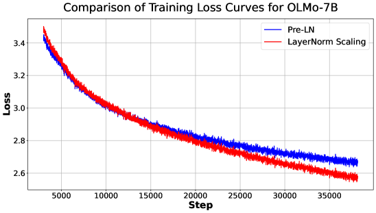![Refer to caption](https://arxiv.org/html/2502.05795v5/x7.png)Figure 6:Training loss of OLMo\-7B with Pre\-LN and LNS\.Loss Curve\.Figure[6](https://arxiv.org/html/2502.05795v5#S5.F6)shows the training loss curves of 7B models trained with Pre\-LN and LNS\. While LayerNorm Scaling exhibits slightly slower convergence at the early stages of training, it consistently outperforms Pre\-LN as training progresses, ultimately achieving a substantial loss gap\. We attribute this to the uncontrolled accumulation of output variance in Pre\-LN, which amplifies with depth and training steps, ultimately impairing the effective learning of deeper layers\. In contrast, LNS mitigates this issue by scaling down the output variance in proportion to depth, thereby enabling more stable and effective training across all layers during training\.

Beating OLMo’s Scaled Initialization\.OLMo adopts the scaled initialization proposed inZhanget al\.\([2019](https://arxiv.org/html/2502.05795v5#bib.bib74)\)and used byMehtaet al\.\([2024](https://arxiv.org/html/2502.05795v5#bib.bib73)\), which scales input projections by1/dmodel1/\\sqrt\{d\_\{\\mathrm\{model\}\}\}, and output projections by1/2⋅dmodel⋅l1/\\sqrt\{2\\cdot d\_\{\\mathrm\{model\}\}\\cdot l\}at every layer\. This method is designed to enhance training stability and to scale down variance at initialization\. To evaluate the effectiveness of LNS, we compare it against this state\-of\-the\-art initialization by training OLMo\-1B on 20B tokens\. As shown in Table[3](https://arxiv.org/html/2502.05795v5#S5.T3), LNS achieves consistently lower training loss, indicating that it may offer a more effective alternative for large\-scale LLM training\.

Table 3:Comparison with OLMo’s Scaled Initialization\.
#### 5\.3\.2Qwen2\.5

We further evaluate the generalizability of LNS by applying it to a state\-of\-the\-art architecture, Qwen2\.5\-0\.5B\(Yanget al\.,[2024](https://arxiv.org/html/2502.05795v5#bib.bib66)\)\. We train the model for 6B tokens and compare LNS against the standard Pre\-LN setup\. Consistent with previous findings, Table[4](https://arxiv.org/html/2502.05795v5#S5.T4)illustrates that LNS yields a notable reduction in perplexity—from 20\.62 to 19\.57—highlighting its effectiveness even on strong, modern architectures\.

Table 4:Perplexity \(PPL↓\\downarrow\) comparison under scaled\-up pre\-training\. For LLaMA\-1B and 7B, training is scheduled for 100B tokens but is terminated early to report results\. Qwen\-2\.5 is trained with a fixed budget of 6B tokens\.The consistent benefits observed across increased model scales, larger training datasets, and diverse architectures suggest that LNS is a promising technique for enhancing the training of contemporary large language models, ensuring that deeper layers contribute more effectively to learning\.

### 5\.4LNS Effectively Scales Down Output Variance

As LNS is proposed to reduce output variance, we empirically validate this claim during the pre\-training of LLMs\. We compare the layerwise output variance of three configurations: \(1\) the standard Pre\-LN\(Ba,[2016](https://arxiv.org/html/2502.05795v5#bib.bib32)\), \(2\) Pre\-LN with Scaled Initialization\(Shoeybiet al\.,[2020](https://arxiv.org/html/2502.05795v5#bib.bib48); Radfordet al\.,[2019](https://arxiv.org/html/2502.05795v5#bib.bib71)\), which scales the initialization of the feedforward layers’ weightsW0W\_\{0\}andW2W\_\{2\}by12​L\\frac\{1\}\{\\sqrt\{2L\}\}, whereLLis the total number of Transformer layers, and \(3\) Pre\-LN with LNS\. The average output variance across layers is shown in Figure[4](https://arxiv.org/html/2502.05795v5#S2.F4)\. For both vanilla Pre\-LN and Scaled Initialization, the output variance in shallow layers \(blue\) remains relatively stable throughout training, while variance in deeper layers \(red\) grows substantially after 2K iterations, reaching up to 175 in the final layer\. Since Scaled Initialization only operates at initialization, it is insufficient to constrain output variance during training\. In contrast, LNS consistently suppresses the growth of output variance in deeper layers, capping it at approximately 25\.

### 5\.5LNS Enhances the Effectiveness of Deep Layers

![Refer to caption](https://arxiv.org/html/2502.05795v5/x8.png)

![Refer to caption](https://arxiv.org/html/2502.05795v5/x9.png)

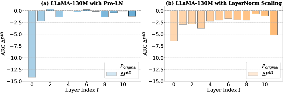
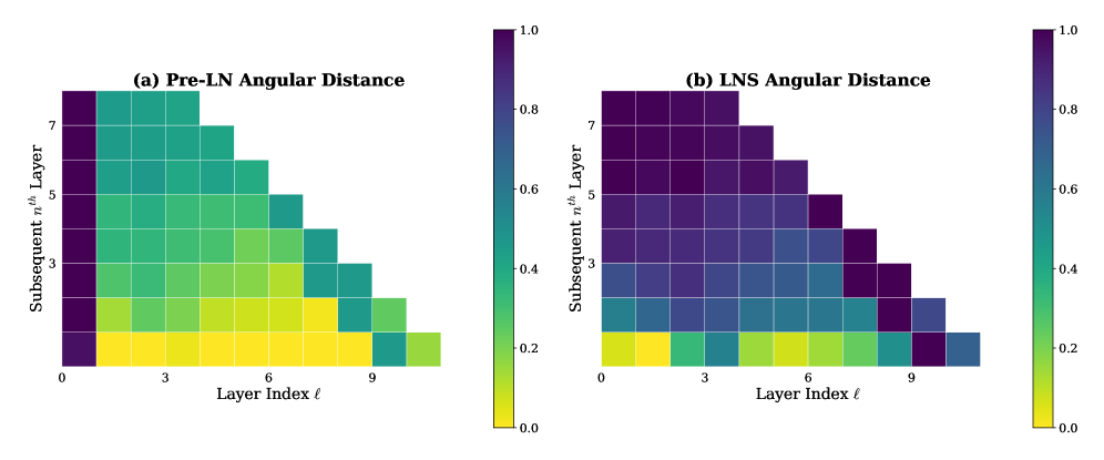
Figure 7:Left:Performance drop of layer pruning on LLaMA\-130M\.Right:The angular distance between representations of subsequent layers is shown\. LayerNorm Scaling enables deep layers to make a meaningful contribution to the model\.Furthermore, to assess whether LNS enhances the effectiveness of deeper layers by promoting more diverse feature representations, we analyze the layerwise performance drop and the angular distance of LNS, as shown in Figure[7](https://arxiv.org/html/2502.05795v5#S5.F7)\. Compared to Pre\-LN, the performance degradation in LayerNorm Scaling is more uniformly distributed across layers, indicating a more balanced contribution from each layer\. Notably, pruning the deeper layers of LNS results in a more significant accuracy drop, suggesting these layers play a more critical role in task performance\. Additionally, features learned under LNS exhibit greater distinction: most layers show a substantial angular distance, exceeding 0\.6, from their adjacent layers, indicating more diverse representations\. In sharp contrast, the layerwise angular distance in Pre\-LN remains significantly lower and progressively decreases with depth, suggesting reduced feature diversity\.

### 5\.6LayerNorm Scaling in Vision Transformer

To evaluate whether LNS also benefits architectures beyond language models, we conduct experiments on ViT\-S on ImageNet\-1K\. Since ViT\-S includes LayerScale\(Touvronet al\.,[2021](https://arxiv.org/html/2502.05795v5#bib.bib25)\)by default—which may interfere with the effect of LNS—we remove LayerScale from all evaluated variants to ensure a fair comparison\. We then test different insertion positions of LNS\. The top\-1 accuracy results are summarized in Table[5](https://arxiv.org/html/2502.05795v5#S5.T5)\. Whereas LNS in language models is typically most effective directly after normalization, in Vision Transformers, the best position is after the attention and MLP blocks\. We next examine whether this performance gain correlates with better control of layer\-wise variance\.

Table 5:Top\-1 accuracy \(%\) of ViT\-S model with and without LNS\.Figure[8](https://arxiv.org/html/2502.05795v5#S5.F8)plots the average output variance of each transformer block during training\. Without LayerScale, variance in deeper layers grows rapidly—exceeding∼3,000\\sim\\\!3\{,\}000by 30K update steps\. Applying LNS after Attn/MLP controls this growth to below∼150\\sim\\\!150, confirming that LNS stabilizes the forward signal even in vision transformers\.

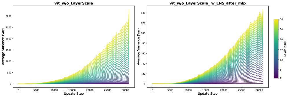![Refer to caption](https://arxiv.org/html/2502.05795v5/x10.png)Figure 8:Layer\-wise output variance of ViT\-SwithoutLayerScale \(left\) and withLNS after Attn/MLP\(right\)\. LNS significantly reduces the variance growth compared to the baseline\.These preliminary findings indicate that the variance\-control mechanism underlying LNS generalizes to vision transformers when the scaling is applied after Attn/MLP\. We leave a more detailed theoretical understanding of this behavior to future work and community discussion\.

## 6Ablation Study

Comparing Against Other Scaling Methods\.We first compare LNS with previous scaling approaches, including \(1\) Scaled Initialization\(Shoeybiet al\.,[2020](https://arxiv.org/html/2502.05795v5#bib.bib48); Radfordet al\.,[2019](https://arxiv.org/html/2502.05795v5#bib.bib71)\), which scales the initialization ofW0W\_\{0\}andW2W\_\{2\}by the overall depth1/2​L1/\\sqrt\{2L\}; \(2\) Depth\-Scaled Initialization\(Zhanget al\.,[2019](https://arxiv.org/html/2502.05795v5#bib.bib74)\)scales the initialization of weight matrices by the current depth1/2​l1/\\sqrt\{2l\}; \(3\) SkipInit\(De and Smith,[2020](https://arxiv.org/html/2502.05795v5#bib.bib4)\)introduces a learnable parameter after FFN/Att layers, initialized as1/L1/\\sqrt\{L\}; \(4\) LayerScale\(Touvronet al\.,[2021](https://arxiv.org/html/2502.05795v5#bib.bib25)\)applies per\-channel weighting using a diagonal matrix,diag\(λ1,…,λd\)\(\\lambda\_\{1\},\\ldots,\\lambda\_\{d\}\), where each weightλi\\lambda\_\{i\}is initialized to a small value \(e\.g\.,λi=ϵ\\lambda\_\{i\}=\\epsilon\)\. Table[6](https://arxiv.org/html/2502.05795v5#S6.T6)presents the results of LLaMA\-130M and LLaMA\-250M\.

First, we observe that methods involving learnable parameters, such as LayerScale and SkipInit, consistently degrade performance in LLMs\. Among initialization\-based techniques, a larger scaling factor proves beneficial: Scaled Initialization yields lower perplexity compared to Depth\-Scaled Initialization\. Notably, LNS achieves the best overall performance, underscoring the advantage of applying scaling dynamically during training\.Interestingly, combining LNS with Scaled Initialization results in worse performance than using LNS alone, highlighting the importance of removing conflicting initialization strategies prior to adopting LNS\.

Table 6:Comparing LNS against other scaling methods\. Perplexity \(↓\) is reported\.Comparison with Other Layer Normalization\.In addition, we conducted comparisons using LLaMA\-130M to evaluate LayerNorm Scaling against recently proposed normalization methods, including Admin\(Liuet al\.,[2020](https://arxiv.org/html/2502.05795v5#bib.bib54)\), Sandwich\-LN\(Dinget al\.,[2021](https://arxiv.org/html/2502.05795v5#bib.bib35)\), Group\-LN\(Wu and He,[2018](https://arxiv.org/html/2502.05795v5#bib.bib37); Maet al\.,[2024](https://arxiv.org/html/2502.05795v5#bib.bib36)\), and Mix\-LN\(Liet al\.,[2024b](https://arxiv.org/html/2502.05795v5#bib.bib76)\)\. Table[7](https://arxiv.org/html/2502.05795v5#S6.T7)shows that Admin and Group\-LN degrade performance\. Sandwich\-LN slightly outperforms Pre\-LN\. Both Mix\-LN and LayerNorm Scaling improve over Pre\-LN by good margins\. However, Mix\-LN fails to reduce perplexity under 26, falling short of LayerNorm Scaling and suffers from instability in large\-scale scenarios as shown in Table[1](https://arxiv.org/html/2502.05795v5#S5.T1)\.

Table 7:Comparison against other normalization methods on LLaMA\-130M\. All methods use the identical configurations\. Perplexity \(↓\) is reported\.Effect of Positions of LNS\.The results in Table[8](https://arxiv.org/html/2502.05795v5#S6.T8)show that inserting the scaling factor at different points can have a considerable influence on the model’s performance\. Placing it after the residual connection \(“After Residual”\) leads to a perplexity of 1358\.11, which indicates training divergence\. In contrast, LNS incorporates the scaling factor after LN achieving the best perplexity of 25\.76, surpassing both the baseline Pre\-LN setting \(26\.73\) and other placements\. This suggests that modifying the LayerNorm to include the scaling factor can enhance training stability and final performance for this model configuration\.

Table 8:Effects of Insertion Position of LayerNorm Scaling on LLaMA\-130M
## 7Related Work

Ineffectiveness of Deeper Layers in Transformers\.The ineffectiveness of deep layers in LLMs has been previously reported\.Yinet al\.\([2024](https://arxiv.org/html/2502.05795v5#bib.bib60)\)found that deeper layers of LLMs can tolerate significantly higher levels of pruning compared to shallower layers, achieving high sparsity\. Similarly,Gromovet al\.\([2024](https://arxiv.org/html/2502.05795v5#bib.bib52)\)andMenet al\.\([2024](https://arxiv.org/html/2502.05795v5#bib.bib10)\)demonstrated that removing early layers causes a dramatic decline in model performance, whereas removing deep layers does not\.Ladet al\.\([2024](https://arxiv.org/html/2502.05795v5#bib.bib40)\)showed that the middle and deep layers of GPT\-2 and Pythia exhibit remarkable robustness to perturbations such as layer swapping and layer dropping\. Recently,Liet al\.\([2024a](https://arxiv.org/html/2502.05795v5#bib.bib51)\)highlighted that early layers contain more outliers and are therefore more critical for fine\-tuning\. While these studies effectively highlight the limitations of deep layers in LLMs, they stop short of identifying the root cause of this issue or proposing viable solutions to address it\.

Layer Normalization in Language Models\.LN\(Ba,[2016](https://arxiv.org/html/2502.05795v5#bib.bib32)\)was initially applied after the residual connection in the original Transformer\(Vaswani,[2017](https://arxiv.org/html/2502.05795v5#bib.bib29)\), which is known as Post\-LN\. Later on, Pre\-LN\(Baevski and Auli,[2019](https://arxiv.org/html/2502.05795v5#bib.bib28); Daiet al\.,[2019](https://arxiv.org/html/2502.05795v5#bib.bib33); Nguyen and Salazar,[2019](https://arxiv.org/html/2502.05795v5#bib.bib34)\)dominated LLMs, due to its compelling performance and stability\(Brownet al\.,[2020](https://arxiv.org/html/2502.05795v5#bib.bib63); Touvronet al\.,[2023](https://arxiv.org/html/2502.05795v5#bib.bib62); Jianget al\.,[2023](https://arxiv.org/html/2502.05795v5#bib.bib14); Biet al\.,[2024](https://arxiv.org/html/2502.05795v5#bib.bib56)\)\. Prior works have studied the effect of Pre\-LN and Post\-LN\.Xionget al\.\([2020](https://arxiv.org/html/2502.05795v5#bib.bib31)\)proves that Post\-LN tends to have larger gradients near the output layer, which necessitates smaller learning rates to stabilize training, whereas Pre\-LN scales down gradients with the depth of the model, working better for deep Transformers\.Wanget al\.\([2019](https://arxiv.org/html/2502.05795v5#bib.bib43)\)empirically confirmed that Pre\-LN facilitates stacking more layers and Post\-LN suffers from gradient vanishing\. The idea of connecting multiple layers was proposed in previous works\(Bapnaet al\.,[2018](https://arxiv.org/html/2502.05795v5#bib.bib42); Douet al\.,[2018](https://arxiv.org/html/2502.05795v5#bib.bib41); Wanget al\.,[2019](https://arxiv.org/html/2502.05795v5#bib.bib43)\)\. Admin introduces additional parameters to control residual dependencies, stabilizing Post\-LN\. DeepNorm\(Wanget al\.,[2024](https://arxiv.org/html/2502.05795v5#bib.bib59)\)enables stacking 1000\-layer Transformers by upscaling the residual connection before applying LN\. Additionally,Dinget al\.\([2021](https://arxiv.org/html/2502.05795v5#bib.bib35)\)proposed Sandwich LayerNorm, normalizing both the input and output of each transformer sub\-layer\.Takaseet al\.\([2023a](https://arxiv.org/html/2502.05795v5#bib.bib53)\)introduced B2T to bypass all LN except the final one in each layer\.Liet al\.\([2024b](https://arxiv.org/html/2502.05795v5#bib.bib76)\)recently combines Post\-LN and Pre\-LN to enhance the middle layers\.Zhuet al\.\([2025b](https://arxiv.org/html/2502.05795v5#bib.bib9)\)introduces Dynamic Tanh \(DyT\) as a normalization\-free alternative in Transformers, delivering comparable performance\.Zhuoet al\.\([2025](https://arxiv.org/html/2502.05795v5#bib.bib2)\)proposes HybridNorm, a hybrid normalization scheme combining QKV normalization with Post\-Norm FFN to stabilize training in deep transformers\.De and Smith \([2020](https://arxiv.org/html/2502.05795v5#bib.bib4)\)also states that normalized residual blocks in deep networks are close to the identity function and proposes SkipInit to remove normalization by introducing a learnable scalar multiplier on the residual branch initialized to1/L1/\\sqrt\{L\}\. Our experiments suggest that SkipInit’s learnable parameter does not improve performance and sometimes harms training\.

## 8Conclusion

In this paper, we re\-introduce the concept of theCurse of Depthin LLMs, highlighting an urgent yet often overlooked phenomenon: nearly half of the deep layers in modern LLMs are less effective than expected\. We discover the root cause of this phenomenon is Pre\-LN which is widely used in almost all modern LLMs\. To tackle this issue, we introduceLayerNorm Scaling\. By scaling the output variance inversely with the layer depth, LayerNorm Scaling ensures that all layers, including deeper ones, contribute meaningfully to training\. Our experiments show that this simple modification improves performance, reduces resource usage, and stabilizes training across various model sizes\. LayerNorm Scaling is easy to implement, hyperparameter\-free, and provides a robust solution to enhance the efficiency and effectiveness of LLMs\.

## References

- J\. Achiam, S\. Adler, S\. Agarwal, L\. Ahmad, I\. Akkaya, F\. L\. Aleman, D\. Almeida, J\. Altenschmidt, S\. Altman, S\. Anadkat,et al\.\(2023\)Gpt\-4 technical report\.arXiv preprint arXiv:2303\.08774\.Cited by:[§1](https://arxiv.org/html/2502.05795v5#S1.p2.1)\.
- Layer normalization\.arXiv preprint arXiv:1607\.06450\.Cited by:[§5\.4](https://arxiv.org/html/2502.05795v5#S5.SS4.p1.4),[Table 1](https://arxiv.org/html/2502.05795v5#S5.T1.4.1.3.1.1),[Table 2](https://arxiv.org/html/2502.05795v5#S5.T2.5.1.3.1.1),[Table 2](https://arxiv.org/html/2502.05795v5#S5.T2.5.1.9.7.1),[§7](https://arxiv.org/html/2502.05795v5#S7.p2.1)\.
- A\. Baevski and M\. Auli \(2019\)Adaptive input representations for neural language modeling\.ICLR\.Cited by:[§1](https://arxiv.org/html/2502.05795v5#S1.p6.1),[§3](https://arxiv.org/html/2502.05795v5#S3.p1.5),[Table 1](https://arxiv.org/html/2502.05795v5#S5.T1.4.1.6.4.1),[Table 2](https://arxiv.org/html/2502.05795v5#S5.T2.5.1.12.10.1),[Table 2](https://arxiv.org/html/2502.05795v5#S5.T2.5.1.6.4.1),[§7](https://arxiv.org/html/2502.05795v5#S7.p2.1)\.
- S\. Bai, K\. Chen, X\. Liu, J\. Wang, W\. Ge, S\. Song, K\. Dang, P\. Wang, S\. Wang, J\. Tang,et al\.\(2025\)Qwen2\. 5\-vl technical report\.arXiv preprint arXiv:2502\.13923\.Cited by:[Appendix C](https://arxiv.org/html/2502.05795v5#A3.p1.1)\.
- A\. Bapna, M\. X\. Chen, O\. Firat, Y\. Cao, and Y\. Wu \(2018\)Training deeper neural machine translation models with transparent attention\.EMNLP\.Cited by:[§7](https://arxiv.org/html/2502.05795v5#S7.p2.1)\.
- X\. Bi, D\. Chen, G\. Chen, S\. Chen, D\. Dai, C\. Deng, H\. Ding, K\. Dong, Q\. Du, Z\. Fu,et al\.\(2024\)Deepseek llm: scaling open\-source language models with longtermism\.arXiv preprint arXiv:2401\.02954\.Cited by:[§2\.1](https://arxiv.org/html/2502.05795v5#S2.SS1.p1.1),[§7](https://arxiv.org/html/2502.05795v5#S7.p2.1)\.
- T\. Brown, B\. Mann, N\. Ryder, M\. Subbiah, J\. D\. Kaplan, P\. Dhariwal, A\. Neelakantan, P\. Shyam, G\. Sastry, A\. Askell,et al\.\(2020\)Language models are few\-shot learners\.NeurIPS\.Cited by:[§7](https://arxiv.org/html/2502.05795v5#S7.p2.1)\.
- Z\. Dai, Z\. Yang, Y\. Yang, J\. Carbonell, Q\. V\. Le, and R\. Salakhutdinov \(2019\)Transformer\-xl: attentive language models beyond a fixed\-length context\.ACL\.Cited by:[§1](https://arxiv.org/html/2502.05795v5#S1.p6.1),[§3](https://arxiv.org/html/2502.05795v5#S3.p1.5),[§5\.1](https://arxiv.org/html/2502.05795v5#S5.SS1.p1.1),[§7](https://arxiv.org/html/2502.05795v5#S7.p2.1)\.
- S\. De and S\. L\. Smith \(2020\)Batch normalization biases residual blocks towards the identity function in deep networks\.External Links:2002\.10444,[Link](https://arxiv.org/abs/2002.10444)Cited by:[Table 6](https://arxiv.org/html/2502.05795v5#S6.T6.4.1.5.2.1),[§6](https://arxiv.org/html/2502.05795v5#S6.p1.8),[§7](https://arxiv.org/html/2502.05795v5#S7.p2.1)\.
- J\. Devlin \(2019\)Bert: pre\-training of deep bidirectional transformers for language understanding\.NAACL\.Cited by:[§2\.1](https://arxiv.org/html/2502.05795v5#S2.SS1.p1.1)\.
- M\. Ding, Z\. Yang, W\. Hong, W\. Zheng, C\. Zhou, D\. Yin, J\. Lin, X\. Zou, Z\. Shao, H\. Yang,et al\.\(2021\)Cogview: mastering text\-to\-image generation via transformers\.NeurIPS34,pp\. 19822–19835\.Cited by:[§6](https://arxiv.org/html/2502.05795v5#S6.p3.1),[§7](https://arxiv.org/html/2502.05795v5#S7.p2.1)\.
- Z\. Dou, Z\. Tu, X\. Wang, S\. Shi, and T\. Zhang \(2018\)Exploiting deep representations for neural machine translation\.EMNLP\.Cited by:[§7](https://arxiv.org/html/2502.05795v5#S7.p2.1)\.
- Z\. Du, Y\. Qian, X\. Liu, M\. Ding, J\. Qiu, Z\. Yang, and J\. Tang \(2021\)Glm: general language model pretraining with autoregressive blank infilling\.arXiv preprint arXiv:2103\.10360\.Cited by:[Appendix D](https://arxiv.org/html/2502.05795v5#A4.SS0.SSS0.Px1.p1.1)\.
- R\. Dumitru, V\. Yadav, R\. Maheshwary, P\. Clotan, S\. T\. Madhusudhan, and M\. Surdeanu \(2024\)Layer\-wise quantization: a pragmatic and effective method for quantizing llms beyond integer bit\-levels\.arXiv preprint arXiv:2406\.17415\.Cited by:[§1](https://arxiv.org/html/2502.05795v5#S1.p1.1)\.
- D\. Groeneveld, I\. Beltagy, P\. Walsh, A\. Bhagia, R\. Kinney, O\. Tafjord, A\. H\. Jha, H\. Ivison, I\. Magnusson, Y\. Wang,et al\.\(2024\)Olmo: accelerating the science of language models\.arXiv preprint arXiv:2402\.00838\.Cited by:[Figure 1](https://arxiv.org/html/2502.05795v5#S0.F1),[Figure 1](https://arxiv.org/html/2502.05795v5#S0.F1.4.1),[§5\.3\.1](https://arxiv.org/html/2502.05795v5#S5.SS3.SSS1.p1.1),[footnote 1](https://arxiv.org/html/2502.05795v5#footnote1)\.
- A\. Gromov, K\. Tirumala, H\. Shapourian, P\. Glorioso, and D\. A\. Roberts \(2024\)The unreasonable ineffectiveness of the deeper layers\.arXiv preprint arXiv:2403\.17887\.Cited by:[§1](https://arxiv.org/html/2502.05795v5#S1.p1.1),[§2\.1](https://arxiv.org/html/2502.05795v5#S2.SS1.p2.1),[§2\.1](https://arxiv.org/html/2502.05795v5#S2.SS1.p4.11),[§7](https://arxiv.org/html/2502.05795v5#S7.p1.1)\.
- D\. Hendrycks, C\. Burns, S\. Basart, A\. Zou, M\. Mazeika, D\. Song, and J\. Steinhardt \(2021\)Measuring massive multitask language understanding\.ICLR\.Cited by:[§1](https://arxiv.org/html/2502.05795v5#S1.p5.1),[§2\.1](https://arxiv.org/html/2502.05795v5#S2.SS1.p3.2)\.
- Z\. Hu, L\. Wang, Y\. Lan, W\. Xu, E\. Lim, L\. Bing, X\. Xu, S\. Poria, and R\. K\. Lee \(2023\)LLM\-adapters: an adapter family for parameter\-efficient fine\-tuning of large language models\.EMNLP\.Cited by:[§5\.2](https://arxiv.org/html/2502.05795v5#S5.SS2.p1.1)\.
- T\. Huang, H\. Hu, Z\. Zhang, G\. Jin, X\. Li, L\. Shen, T\. Chen, L\. Liu, Q\. Wen, Z\. Wang,et al\.\(2025a\)Stable\-spam: how to train in 4\-bit more stably than 16\-bit adam\.arXiv preprint arXiv:2502\.17055\.Cited by:[§A\.1\.2](https://arxiv.org/html/2502.05795v5#A1.SS1.SSS2.p15.1)\.
- T\. Huang, Z\. Zhu, G\. Jin, L\. Liu, Z\. Wang, and S\. Liu \(2025b\)SPAM: spike\-aware adam with momentum reset for stable llm training\.arXiv preprint arXiv:2501\.06842\.Cited by:[§A\.1\.2](https://arxiv.org/html/2502.05795v5#A1.SS1.SSS2.p15.1)\.
- A\. Q\. Jiang, A\. Sablayrolles, A\. Mensch, C\. Bamford, D\. S\. Chaplot, D\. d\. l\. Casas, F\. Bressand, G\. Lengyel, G\. Lample, L\. Saulnier,et al\.\(2023\)Mistral 7b\.arXiv preprint arXiv:2310\.06825\.Cited by:[§7](https://arxiv.org/html/2502.05795v5#S7.p2.1)\.
- D\. P\. Kingma \(2015\)Adam: a method for stochastic optimization\.ICLR\.Cited by:[§5\.1](https://arxiv.org/html/2502.05795v5#S5.SS1.p2.3)\.
- V\. Lad, W\. Gurnee, and M\. Tegmark \(2024\)The remarkable robustness of llms: stages of inference?\.arXiv preprint arXiv:2406\.19384\.Cited by:[§7](https://arxiv.org/html/2502.05795v5#S7.p1.1)\.
- M\. Ledoux \(2001\)The concentration of measure phenomenon\.Mathematical Surveys and Monographs, Vol\.89,American Mathematical Society,Providence, RI\.Cited by:[Lemma A\.1](https://arxiv.org/html/2502.05795v5#A1.Thmtheorem1)\.
- P\. Li, L\. Yin, X\. Gao, and S\. Liu \(2024a\)OwLore: outlier\-weighed layerwise sampled low\-rank projection for memory\-efficient llm fine\-tuning\.arXiv preprint arXiv:2405\.18380\.Cited by:[§7](https://arxiv.org/html/2502.05795v5#S7.p1.1)\.
- P\. Li, L\. Yin, and S\. Liu \(2024b\)Mix\-ln: unleashing the power of deeper layers by combining pre\-ln and post\-ln\.arXiv preprint arXiv:2412\.13795\.Cited by:[§1](https://arxiv.org/html/2502.05795v5#S1.p1.1),[§1](https://arxiv.org/html/2502.05795v5#S1.p2.1),[§1](https://arxiv.org/html/2502.05795v5#S1.p7.1),[§2\.1](https://arxiv.org/html/2502.05795v5#S2.SS1.p2.1),[§2\.2](https://arxiv.org/html/2502.05795v5#S2.SS2.p1.1),[§2](https://arxiv.org/html/2502.05795v5#S2.p1.1),[§4](https://arxiv.org/html/2502.05795v5#S4.p2.6),[§5\.1](https://arxiv.org/html/2502.05795v5#S5.SS1.p1.1),[§5\.1](https://arxiv.org/html/2502.05795v5#S5.SS1.p2.3),[§5\.2](https://arxiv.org/html/2502.05795v5#S5.SS2.p1.1),[Table 1](https://arxiv.org/html/2502.05795v5#S5.T1.4.1.5.3.1),[Table 2](https://arxiv.org/html/2502.05795v5#S5.T2.5.1.11.9.1),[Table 2](https://arxiv.org/html/2502.05795v5#S5.T2.5.1.5.3.1),[§6](https://arxiv.org/html/2502.05795v5#S6.p3.1),[§7](https://arxiv.org/html/2502.05795v5#S7.p2.1)\.
- V\. Lialin, S\. Muckatira, N\. Shivagunde, and A\. Rumshisky \(2023\)Relora: high\-rank training through low\-rank updates\.InICLR,Cited by:[§5\.1](https://arxiv.org/html/2502.05795v5#S5.SS1.p1.1)\.
- L\. Liu, X\. Liu, J\. Gao, W\. Chen, and J\. Han \(2020\)Understanding the difficulty of training transformers\.EMNLP\.Cited by:[§1](https://arxiv.org/html/2502.05795v5#S1.p7.1),[§4](https://arxiv.org/html/2502.05795v5#S4.p2.6),[§6](https://arxiv.org/html/2502.05795v5#S6.p3.1)\.
- H\. Lu, Y\. Zhou, S\. Liu, Z\. Wang, M\. W\. Mahoney, and Y\. Yang \(2024\)Alphapruning: using heavy\-tailed self regularization theory for improved layer\-wise pruning of large language models\.NeurIPS\.Cited by:[§1](https://arxiv.org/html/2502.05795v5#S1.p1.1)\.
- X\. Ma, X\. Yang, W\. Xiong, B\. Chen, L\. Yu, H\. Zhang, J\. May, L\. Zettlemoyer, O\. Levy, and C\. Zhou \(2024\)Megalodon: efficient llm pretraining and inference with unlimited context length\.NeurIPS\.Cited by:[§6](https://arxiv.org/html/2502.05795v5#S6.p3.1)\.
- S\. Mehta, M\. H\. Sekhavat, Q\. Cao, M\. Horton, Y\. Jin, C\. Sun, I\. Mirzadeh, M\. Najibi, D\. Belenko, P\. Zatloukal,et al\.\(2024\)Openelm: an efficient language model family with open training and inference framework\.arXiv preprint arXiv:2404\.14619\.Cited by:[§5\.3\.1](https://arxiv.org/html/2502.05795v5#S5.SS3.SSS1.p3.2)\.
- X\. Men, M\. Xu, Q\. Zhang, B\. Wang, H\. Lin, Y\. Lu, X\. Han, and W\. Chen \(2024\)Shortgpt: layers in large language models are more redundant than you expect\.arXiv preprint arXiv:2403\.03853\.Cited by:[§1](https://arxiv.org/html/2502.05795v5#S1.p1.1),[§7](https://arxiv.org/html/2502.05795v5#S7.p1.1)\.
- S\. Muralidharan, S\. T\. Sreenivas, R\. B\. Joshi, M\. Chochowski, M\. Patwary, M\. Shoeybi, B\. Catanzaro, J\. Kautz, and P\. Molchanov \(2024\)Compact language models via pruning and knowledge distillation\.InNeurIPS,Cited by:[§1](https://arxiv.org/html/2502.05795v5#S1.p1.1)\.
- T\. Q\. Nguyen and J\. Salazar \(2019\)Transformers without tears: improving the normalization of self\-attention\.IWSLT\.Cited by:[§4](https://arxiv.org/html/2502.05795v5#S4.p2.6),[§5\.1](https://arxiv.org/html/2502.05795v5#S5.SS1.p1.1),[§7](https://arxiv.org/html/2502.05795v5#S7.p2.1)\.
- A\. Radford, J\. Wu, R\. Child, D\. Luan, D\. Amodei, I\. Sutskever,et al\.\(2019\)Language models are unsupervised multitask learners\.OpenAI blog1\(8\),pp\. 9\.Cited by:[Figure 4](https://arxiv.org/html/2502.05795v5#S2.F4),[Figure 4](https://arxiv.org/html/2502.05795v5#S2.F4.4.2),[§5\.4](https://arxiv.org/html/2502.05795v5#S5.SS4.p1.4),[§6](https://arxiv.org/html/2502.05795v5#S6.p1.8),[footnote 1](https://arxiv.org/html/2502.05795v5#footnote1)\.
- P\. Rajpurkar \(2016\)Squad: 100,000\+ questions for machine comprehension of text\.EMNLP\.Cited by:[§2\.1](https://arxiv.org/html/2502.05795v5#S2.SS1.p3.2)\.
- N\. Shazeer \(2020\)Glu variants improve transformer\.arXiv preprint arXiv:2002\.05202\.Cited by:[§5\.1](https://arxiv.org/html/2502.05795v5#S5.SS1.p2.3)\.
- M\. Shoeybi, M\. Patwary, R\. Puri, P\. LeGresley, J\. Casper, and B\. Catanzaro \(2020\)Megatron\-lm: training multi\-billion parameter language models using model parallelism\.ICML\.Cited by:[Figure 4](https://arxiv.org/html/2502.05795v5#S2.F4),[Figure 4](https://arxiv.org/html/2502.05795v5#S2.F4.4.2),[§5\.4](https://arxiv.org/html/2502.05795v5#S5.SS4.p1.4),[Table 6](https://arxiv.org/html/2502.05795v5#S6.T6.4.1.7.4.1),[§6](https://arxiv.org/html/2502.05795v5#S6.p1.8),[footnote 1](https://arxiv.org/html/2502.05795v5#footnote1)\.
- S\. A\. Siddiqui, X\. Dong, G\. Heinrich, T\. Breuel, J\. Kautz, D\. Krueger, and P\. Molchanov \(2024\)A deeper look at depth pruning of llms\.ICML\.Cited by:[§1](https://arxiv.org/html/2502.05795v5#S1.p1.1)\.
- S\. Takase, S\. Kiyono, S\. Kobayashi, and J\. Suzuki \(2023a\)B2t connection: serving stability and performance in deep transformers\.ACL\.Cited by:[§7](https://arxiv.org/html/2502.05795v5#S7.p2.1)\.
- S\. Takase, S\. Kiyono, S\. Kobayashi, and J\. Suzuki \(2023b\)Spike no more: stabilizing the pre\-training of large language models\.arXiv preprint arXiv:2312\.16903\.Cited by:[§A\.1](https://arxiv.org/html/2502.05795v5#A1.SS1.1.p1.1),[§A\.2\.1](https://arxiv.org/html/2502.05795v5#A1.SS2.SSS1.1.p1.1),[§A\.2\.2](https://arxiv.org/html/2502.05795v5#A1.SS2.SSS2.p1.6),[§3\.1](https://arxiv.org/html/2502.05795v5#S3.SS1.p2.1),[§4\.1](https://arxiv.org/html/2502.05795v5#S4.SS1.p5.1)\.
- Q\. Team \(2025\)Note:Accessed: 2025\-05\-11External Links:[Link](https://qwenlm.github.io/blog/qwen3/)Cited by:[§2\.1](https://arxiv.org/html/2502.05795v5#S2.SS1.p1.1)\.
- H\. Touvron, M\. Cord, A\. Sablayrolles, G\. Synnaeve, and H\. Jégou \(2021\)Going deeper with image transformers\.InICCV,pp\. 32–42\.Cited by:[§5\.6](https://arxiv.org/html/2502.05795v5#S5.SS6.p1.1),[Table 6](https://arxiv.org/html/2502.05795v5#S6.T6.4.1.4.1.1),[§6](https://arxiv.org/html/2502.05795v5#S6.p1.8)\.
- H\. Touvron, T\. Lavril, G\. Izacard, X\. Martinet, M\. Lachaux, T\. Lacroix, B\. Rozière, N\. Goyal, E\. Hambro, F\. Azhar,et al\.\(2023\)Llama: open and efficient foundation language models\.arXiv preprint arXiv:2302\.13971\.Cited by:[§1](https://arxiv.org/html/2502.05795v5#S1.p2.1),[§2\.1](https://arxiv.org/html/2502.05795v5#S2.SS1.p1.1),[§7](https://arxiv.org/html/2502.05795v5#S7.p2.1)\.
- A\. Vaswani \(2017\)Attention is all you need\.NeurIPS\.Cited by:[§7](https://arxiv.org/html/2502.05795v5#S7.p2.1)\.
- R\. Vershynin \(2018\)High\-dimensional probability: an introduction with applications in data science\.Cambridge Series in Statistical and Probabilistic Mathematics,Cambridge University Press\.Cited by:[§A\.2\.1](https://arxiv.org/html/2502.05795v5#A1.SS2.SSS1.3.p3.6),[§A\.2\.1](https://arxiv.org/html/2502.05795v5#A1.SS2.SSS1.8.p8.7),[§A\.5](https://arxiv.org/html/2502.05795v5#A1.SS5.4.p4.1)\.
- H\. Wang, S\. Ma, L\. Dong, S\. Huang, D\. Zhang, and F\. Wei \(2024\)Deepnet: scaling transformers to 1,000 layers\.TPAMI\.Cited by:[§A\.1\.2](https://arxiv.org/html/2502.05795v5#A1.SS1.SSS2.p4.1),[§4](https://arxiv.org/html/2502.05795v5#S4.p2.6),[§5\.1](https://arxiv.org/html/2502.05795v5#S5.SS1.p1.1),[Table 1](https://arxiv.org/html/2502.05795v5#S5.T1.4.1.4.2.1),[Table 2](https://arxiv.org/html/2502.05795v5#S5.T2.5.1.10.8.1),[Table 2](https://arxiv.org/html/2502.05795v5#S5.T2.5.1.4.2.1),[§7](https://arxiv.org/html/2502.05795v5#S7.p2.1)\.
- Q\. Wang, B\. Li, T\. Xiao, J\. Zhu, C\. Li, D\. F\. Wong, and L\. S\. Chao \(2019\)Learning deep transformer models for machine translation\.ACL\.Cited by:[§7](https://arxiv.org/html/2502.05795v5#S7.p2.1)\.
- E\. T\. Whittaker and G\. N\. Watson \(1996\)A course of modern analysis\.4 edition,Cambridge Mathematical Library,Cambridge University Press\.Cited by:[§A\.2\.2](https://arxiv.org/html/2502.05795v5#A1.SS2.SSS2.p3.1),[§A\.4](https://arxiv.org/html/2502.05795v5#A1.SS4.5.p5.1)\.
- Y\. Wu and K\. He \(2018\)Group normalization\.InECCV,pp\. 3–19\.Cited by:[§6](https://arxiv.org/html/2502.05795v5#S6.p3.1)\.
- R\. Xiong, Y\. Yang, D\. He, K\. Zheng, S\. Zheng, C\. Xing, H\. Zhang, Y\. Lan, L\. Wang, and T\. Liu \(2020\)On layer normalization in the transformer architecture\.InICML,pp\. 10524–10533\.Cited by:[§7](https://arxiv.org/html/2502.05795v5#S7.p2.1)\.
- A\. Yang, B\. Yang, B\. Zhang, B\. Hui, B\. Zheng, B\. Yu, C\. Li, D\. Liu, F\. Huang, H\. Wei, H\. Lin, J\. Yang, J\. Tu, J\. Zhang, J\. Yang, J\. Yang, J\. Zhou, J\. Lin, K\. Dang, K\. Lu, K\. Bao, K\. Yang, L\. Yu, M\. Li, M\. Xue, P\. Zhang, Q\. Zhu, R\. Men, R\. Lin, T\. Li, T\. Xia, X\. Ren, X\. Ren, Y\. Fan, Y\. Su, Y\. Zhang, Y\. Wan, Y\. Liu, Z\. Cui, Z\. Zhang, and Z\. Qiu \(2024\)Qwen2\.5 technical report\.arXiv preprint arXiv:2412\.15115\.Cited by:[§5\.3\.2](https://arxiv.org/html/2502.05795v5#S5.SS3.SSS2.p1.1)\.
- G\. Yang, D\. Yu, C\. Zhu, and S\. Hayou \(2023\)Tensor programs vi: feature learning in infinite\-depth neural networks\.arXiv preprint arXiv:2310\.02244\.Cited by:[§2\.1](https://arxiv.org/html/2502.05795v5#S2.SS1.p4.11)\.
- L\. Yin, Y\. Wu, Z\. Zhang, C\. Hsieh, Y\. Wang, Y\. Jia, M\. Pechenizkiy, Y\. Liang, Z\. Wang, and S\. Liu \(2024\)Outlier weighed layerwise sparsity \(owl\): a missing secret sauce for pruning llms to high sparsity\.ICML\.Cited by:[§1](https://arxiv.org/html/2502.05795v5#S1.p1.1),[§7](https://arxiv.org/html/2502.05795v5#S7.p1.1)\.
- X\. Yue, Y\. Ni, K\. Zhang, T\. Zheng, R\. Liu, G\. Zhang, S\. Stevens, D\. Jiang, W\. Ren, Y\. Sun,et al\.\(2024\)Mmmu: a massive multi\-discipline multimodal understanding and reasoning benchmark for expert agi\.InProceedings of the IEEE/CVF Conference on Computer Vision and Pattern Recognition,pp\. 9556–9567\.Cited by:[Appendix C](https://arxiv.org/html/2502.05795v5#A3.p1.1)\.
- B\. Zhang and R\. Sennrich \(2019\)Root mean square layer normalization\.NeurIPS32\.Cited by:[§5\.1](https://arxiv.org/html/2502.05795v5#S5.SS1.p2.3)\.
- B\. Zhang, I\. Titov, and R\. Sennrich \(2019\)Improving deep transformer with depth\-scaled initialization and merged attention\.arXiv preprint arXiv:1908\.11365\.Cited by:[§5\.3\.1](https://arxiv.org/html/2502.05795v5#S5.SS3.SSS1.p3.2),[Table 6](https://arxiv.org/html/2502.05795v5#S6.T6.4.1.6.3.1),[§6](https://arxiv.org/html/2502.05795v5#S6.p1.8)\.
- J\. Zhao, Z\. Zhang, B\. Chen, Z\. Wang, A\. Anandkumar, and Y\. Tian \(2024\)Galore: memory\-efficient llm training by gradient low\-rank projection\.ICML\.Cited by:[§5\.1](https://arxiv.org/html/2502.05795v5#S5.SS1.p1.1)\.
- J\. Zhu, X\. Chen, K\. He, Y\. LeCun, and Z\. Liu \(2025a\)Transformers without normalization\.arXiv preprint arXiv:2503\.10622\.Cited by:[Appendix D](https://arxiv.org/html/2502.05795v5#A4.SS0.SSS0.Px1.p1.1)\.
- J\. Zhu, X\. Chen, K\. He, Y\. LeCun, and Z\. Liu \(2025b\)Transformers without normalization\.External Links:2503\.10622,[Link](https://arxiv.org/abs/2503.10622)Cited by:[§7](https://arxiv.org/html/2502.05795v5#S7.p2.1)\.
- Z\. Zhuo, Y\. Zeng, Y\. Wang, S\. Zhang, J\. Yang, X\. Li, X\. Zhou, and J\. Ma \(2025\)HybridNorm: towards stable and efficient transformer training via hybrid normalization\.External Links:2503\.04598,[Link](https://arxiv.org/abs/2503.04598)Cited by:[§7](https://arxiv.org/html/2502.05795v5#S7.p2.1)\.

## Appendix AProofs of the Theorems of curse of depth

### A\.1Proof of Lemma[3\.2](https://arxiv.org/html/2502.05795v5#S3.Thmtheorem2)

###### Proof\.

Given Equation \([2](https://arxiv.org/html/2502.05795v5#S3.E2)\) fromTakaseet al\.\([2023b](https://arxiv.org/html/2502.05795v5#bib.bib38)\), we have:

y\\displaystyle y=xℓ\+1=xℓ′\+FFN​\(LN​\(xℓ′\)\),\\displaystyle=x\_\{\\ell\+1\}=x^\{\\prime\}\_\{\\ell\}\+\\mathrm\{FFN\}\(\\mathrm\{LN\}\(x^\{\\prime\}\_\{\\ell\}\)\),\(20\)xℓ′\\displaystyle x^\{\\prime\}\_\{\\ell\}=xℓ\+Attn​\(LN​\(xℓ\)\)\.\\displaystyle=x\_\{\\ell\}\+\\mathrm\{Attn\}\(\\mathrm\{LN\}\(x\_\{\\ell\}\)\)\.
Based on our Assumption[3\.1](https://arxiv.org/html/2502.05795v5#S3.Thmtheorem1), letVar​\(Attn​\(LN​\(xℓ\)\)\)=σAttn2\\mathrm\{Var\}\(\\mathrm\{Attn\}\(\\mathrm\{LN\}\(x\_\{\\ell\}\)\)\)=\\sigma\_\{\\text\{Attn\}\}^\{2\}\. Then we can write:

Var​\(xℓ′\)\\displaystyle\\mathrm\{Var\}\(x^\{\\prime\}\_\{\\ell\}\)=Var​\(xℓ\)\+Var​\(Attn​\(LN​\(xℓ\)\)\)\+Cov​\(Attn​\(LN​\(xℓ\)\),Var​\(xℓ\)\)\\displaystyle=\\mathrm\{Var\}\(x\_\{\\ell\}\)\+\\mathrm\{Var\}\(\\mathrm\{Attn\}\(\\mathrm\{LN\}\(x\_\{\\ell\}\)\)\)\+\\mathrm\{Cov\}\(\\mathrm\{Attn\}\(\\mathrm\{LN\}\(x\_\{\\ell\}\)\),\\mathrm\{Var\}\(x\_\{\\ell\}\)\)\(21\)=σxℓ2\+σAttn2\+ρ1⋅σxℓ⋅σAttn,\\displaystyle=\\sigma\_\{x\_\{\\ell\}\}^\{2\}\+\\sigma\_\{\\text\{Attn\}\}^\{2\}\+\\rho\_\{1\}\\cdot\\sigma\_\{x\_\{\\ell\}\}\\cdot\\sigma\_\{\\text\{Attn\}\},
whereρ1\\rho\_\{1\}is the correlation factor\. Similarly, letVar​\(FFN​\(LN​\(xℓ′\)\)\)=σFFN2\\mathrm\{Var\}\(\\mathrm\{FFN\}\(\\mathrm\{LN\}\(x^\{\\prime\}\_\{\\ell\}\)\)\)=\\sigma\_\{\\mathrm\{FFN\}\}^\{2\}\. Then we have:

σxℓ\+12=σ\(xℓ′\)2\+σFFN2\+ρ2⋅σxℓ′⋅σFFN,\\sigma^\{2\}\_\{x\_\{\\ell\+1\}\}=\\sigma\_\{\(\}x^\{\\prime\}\_\{\\ell\}\)^\{2\}\+\\sigma\_\{\\mathrm\{FFN\}\}^\{2\}\+\\rho\_\{2\}\\cdot\\sigma\_\{x^\{\\prime\}\_\{\\ell\}\}\\cdot\\sigma\_\{\\mathrm\{FFN\}\},\(22\)
whereρ2\\rho\_\{2\}is the correlation factor\. Thus, the relationship betweenVar​\(xℓ\+1\)\\mathrm\{Var\}\(x\_\{\\ell\+1\}\)andVar​\(xℓ\)\\mathrm\{Var\}\(x\_\{\\ell\}\)becomes:

σxℓ\+12=σxℓ2\+σAttn2\+σFFN2\+ρ1⋅σxℓ⋅σAttn\+ρ2⋅σxℓ′⋅σFFN\.\\sigma^\{2\}\_\{x\_\{\\ell\+1\}\}=\\sigma^\{2\}\_\{x\_\{\\ell\}\}\+\\sigma\_\{\\text\{Attn\}\}^\{2\}\+\\sigma\_\{\\mathrm\{FFN\}\}^\{2\}\+\\rho\_\{1\}\\cdot\\sigma\_\{x\_\{\\ell\}\}\\cdot\\sigma\_\{\\text\{Attn\}\}\+\\rho\_\{2\}\\cdot\\sigma\_\{x^\{\\prime\}\_\{\\ell\}\}\\cdot\\sigma\_\{\\mathrm\{FFN\}\}\.\(23\)

#### A\.1\.1Variance of the Attention

The scaled dot\-product attention mechanism is defined as:

Attn​\(Q,K,V\)=softmax​\(Q​KTdk\)​V\.\\mathrm\{Attn\}\(Q,K,V\)=\\mathrm\{softmax\}\\left\(\\frac\{QK^\{T\}\}\{\\sqrt\{d\_\{k\}\}\}\\right\)V\.\(24\)
The softmax function outputs a probability distribution over the keys\. Let the softmax output beA=softmax​\(Q​KTdk\)A=\\mathrm\{softmax\}\\left\(\\frac\{QK^\{T\}\}\{\\sqrt\{d\_\{k\}\}\}\\right\), whereAAis a matrix with each row summing to 1\. The final attention output is obtained by multiplying the softmax outputAAwith the value matrixVV:

Attn​\(Q,K,V\)=A​V\.\\mathrm\{Attn\}\(Q,K,V\)=AV\.\(25\)
###### Lemma A\.1\(Ledoux \([2001](https://arxiv.org/html/2502.05795v5#bib.bib11)\)\)\.

Let\{Xi\}i=1N\\\{X\_\{i\}\\\}\_\{i=1\}^\{N\}be independent and identically distributed random variables with meanmmand varianceσ2<∞\\sigma^\{2\}<\\infty\. Define the softmax weightspi=eXi∑j=1NeXj,and letp=\(p1,…,pN\)\.p\_\{i\}=\\frac\{e^\{X\_\{i\}\}\}\{\\sum\_\{j=1\}^\{N\}e^\{X\_\{j\}\}\},\\quad\\text\{and let\}\\quad p=\(p\_\{1\},\\ldots,p\_\{N\}\)\.Then, asN→∞N\\to\\infty, with high probability, the softmax vectorppconcentrates around the uniform distribution onNNelements\. In particular,

limn→∞𝔼​\[∑i=1N\(pi−1n\)2\]=0,\\lim\_\{n\\rightarrow\\infty\}\\mathbb\{E\}\\left\[\\sum\_\{i=1\}^\{N\}\\left\(p\_\{i\}\-\\frac\{1\}\{n\}\\right\)^\{2\}\\right\]=0,\(26\)which implies that the softmax output becomes asymptotically indistinguishable, in expectation, from the uniform distribution\.

According to the above lemma, to simplify the analysis, we make the following additional assumptions: The softmax outputAAis approximately uniform, meaning each element ofAAis roughly1/n1/n, wherennis the number of keys/values\. Given this assumption, the variance of the attention is:

Var​\(Attn​\(Q,K,V\)\)∼Var​\(A​V\)=1n​∑i=1ndhead​Var​\(Vi\)=1n⋅n​σV2⋅dhead=dhead​σV2=σW2​d\.\\mathrm\{Var\}\(\\mathrm\{Attn\}\(Q,K,V\)\)\\sim\\mathrm\{Var\}\(AV\)=\\frac\{1\}\{n\}\\sum\_\{i=1\}^\{n\}d\_\{\\mathrm\{head\}\}\\mathrm\{Var\}\(V\_\{i\}\)=\\frac\{1\}\{n\}\\cdot n\\sigma\_\{V\}^\{2\}\\cdot d\_\{\\mathrm\{head\}\}=d\_\{\\mathrm\{head\}\}\\sigma\_\{V\}^\{2\}=\\sigma\_\{W\}^\{2\}d\.\(27\)whereWWis the universal weight matrix defined as before\.

#### A\.1\.2Variance of the Feed\-Forward Network

The feed\-forward network \(FFN\) in transformers typically consists of two linear transformations with a ReLU activation in between\. The FFN can be written as:

FFN​\(x\)=W2⋅ReLU​\(W1⋅x\+b1\)\+b2\.\\mathrm\{FFN\}\(x\)=W\_\{2\}\\cdot\\mathrm\{ReLU\}\(W\_\{1\}\\cdot x\+b\_\{1\}\)\+b\_\{2\}\.\(28\)
whereW1W\_\{1\}andW2W\_\{2\}are weight matrices, andb1b\_\{1\}andb2b\_\{2\}are bias vectors\.

Using the result obtained byWanget al\.\([2024](https://arxiv.org/html/2502.05795v5#bib.bib59)\), we get:

σFFN2∼σW12⋅σW22=σW4\.\\sigma\_\{\\mathrm\{FFN\}\}^\{2\}\\sim\\sigma\_\{W\_\{1\}\}^\{2\}\\cdot\\sigma\_\{W\_\{2\}\}^\{2\}=\\sigma\_\{W\}^\{4\}\.\(29\)
In conclusion:

σxℓ′2\\displaystyle\\sigma^\{2\}\_\{x^\{\\prime\}\_\{\\ell\}\}=σxℓ2\+σW2\+ρ2⋅σxℓ⋅σW\\displaystyle=\\sigma\_\{x\_\{\\ell\}\}^\{2\}\+\\sigma\_\{W\}^\{2\}\+\\rho\_\{2\}\\cdot\\sigma\_\{x\_\{\\ell\}\}\\cdot\\sigma\_\{W\}\(30\)=σxℓ2​\(1\+σWσxℓ\+σW2σxℓ2\)\\displaystyle=\\sigma\_\{x\_\{\\ell\}\}^\{2\}\(1\+\\frac\{\\sigma\_\{W\}\}\{\\sigma\_\{x\_\{\\ell\}\}\}\+\\frac\{\\sigma\_\{W\}^\{2\}\}\{\\sigma^\{2\}\_\{x\_\{\\ell\}\}\}\)=σxℓ2​Θ​\(1\+1σxℓ\)\.\\displaystyle=\\sigma\_\{x\_\{\\ell\}\}^\{2\}\\Theta\(1\+\\frac\{1\}\{\\sigma\_\{x\_\{\\ell\}\}\}\)\.For simplicity, we set the numerator part to 1\. Substituteσxℓ′=σxℓ​1\+σW2σxℓ2\+ρ2⋅σWσxℓ\.\\sigma\_\{x^\{\\prime\}\_\{\\ell\}\}=\\sigma\_\{x\_\{\\ell\}\}\\sqrt\{1\+\\frac\{\\sigma\_\{W\}^\{2\}\}\{\\sigma\_\{x\_\{\\ell\}\}^\{2\}\}\+\\rho\_\{2\}\\cdot\\frac\{\\sigma\_\{W\}\}\{\\sigma\_\{x\_\{\\ell\}\}\}\}\.into Equation \([23](https://arxiv.org/html/2502.05795v5#A1.E23)\) we get:

σxℓ\+12\\displaystyle\\sigma^\{2\}\_\{x\_\{\\ell\+1\}\}=σxℓ2\+σW2\+σW4​d2\+ρ1⋅σxℓ⋅σW\+ρ2⋅σxℓ′⋅σW2​d\\displaystyle=\\sigma^\{2\}\_\{x\_\{\\ell\}\}\+\\sigma\_\{W\}^\{2\}\+\\sigma\_\{W\}^\{4\}d^\{2\}\+\\rho\_\{1\}\\cdot\\sigma\_\{x\_\{\\ell\}\}\\cdot\\sigma\_\{W\}\+\\rho\_\{2\}\\cdot\\sigma\_\{x^\{\\prime\}\_\{\\ell\}\}\\cdot\\sigma\_\{W\}^\{2\}d\(31\)=σxℓ2\+σW2\+σW4​d2\+ρ1⋅σxℓ⋅σW\+ρ2⋅σxℓ⋅σW2​d\+ρ2​σW4​d22​σxℓ\+ρ22​σW3​d​σxℓ2\\displaystyle=\\sigma^\{2\}\_\{x\_\{\\ell\}\}\+\\sigma\_\{W\}^\{2\}\+\\sigma\_\{W\}^\{4\}d^\{2\}\+\\rho\_\{1\}\\cdot\\sigma\_\{x\_\{\\ell\}\}\\cdot\\sigma\_\{W\}\+\\rho\_\{2\}\\cdot\\sigma\_\{x\_\{\\ell\}\}\\cdot\\sigma\_\{W\}^\{2\}d\+\\frac\{\\rho\_\{2\}\\sigma\_\{W\}^\{4\}d^\{2\}\}\{2\\sigma\_\{x\_\{\\ell\}\}\}\+\\frac\{\\rho\_\{2\}^\{2\}\\sigma\_\{W\}^\{3\}d\\sigma\_\{x\_\{\\ell\}\}\}\{2\}=σxℓ2​Θ​\(1\+1σxℓ\)\.\\displaystyle=\\sigma\_\{x\_\{\\ell\}\}^\{2\}\\Theta\(1\+\\frac\{1\}\{\\sigma\_\{x\_\{\\ell\}\}\}\)\.
From the result we can generally infer that the variance accumulates layer by layer\. The variance with regard toσx1\\sigma\_\{x\_\{1\}\}:

σxℓ2=σx12​Θ​\(∏k=1ℓ−1\(1\+1σxk\)\)\.\\sigma^\{2\}\_\{x\_\{\\ell\}\}=\\sigma\_\{x\_\{1\}\}^\{2\}\\Theta\\Bigl\(\\prod\_\{k=1\}^\{\\ell\-1\}\\left\(1\+\\frac\{1\}\{\\sigma\_\{x\_\{k\}\}\}\\right\)\\Bigr\)\.\(32\)We can also obtain a similar result forσxℓ′2\\sigma^\{2\}\_\{x^\{\\prime\}\_\{\\ell\}\}\.

We observe that for anyσxk2≥1\{\\sigma^\{2\}\_\{x\_\{k\}\}\}\\geq 1, the sequence is increasing, meaning each term in the product is bounded\. Consequently, the entire product is bounded above by:

σxℓ2≤σx12​∏k=1ℓ−1\(1\+1σx1\)=σx12​\(1\+1σx1\)ℓ−1=exp⁡Θ​\(L\)\.\{\\sigma^\{2\}\_\{x\_\{\\ell\}\}\}\\leq\{\\sigma^\{2\}\_\{x\_\{1\}\}\}\\prod\_\{k=1\}^\{\\ell\-1\}\\Bigl\(1\+\\sqrt\{\\frac\{1\}\{\\sigma\_\{x\_\{1\}\}\}\}\\Bigr\)=\\sigma^\{2\}\_\{x\_\{1\}\}\\bigl\(1\+\\sqrt\{\\frac\{1\}\{\\sigma\_\{x\_\{1\}\}\}\}\\Bigr\)^\{\\ell\-1\}=\\exp\{\\Theta\(L\)\}\.\(33\)
Taking the natural logarithm of both sides:

log⁡\(σxℓ2\)\\displaystyle\\log\(\{\\sigma^\{2\}\_\{x\_\{\\ell\}\}\}\)=log⁡\(σx12​∏k=1ℓ−1\(1\+1σxk2\)\)=∑k=1ℓ−1log⁡\(1\+1σxk2\)\+log⁡\(σx12\)\\displaystyle=\\log\\left\(\\sigma\_\{x\_\{1\}\}^\{2\}\\prod\_\{k=1\}^\{\\ell\-1\}\\left\(1\+\\sqrt\{\\frac\{1\}\{\{\\sigma^\{2\}\_\{x\_\{k\}\}\}\}\}\\right\)\\right\)=\\sum\_\{k=1\}^\{\\ell\-1\}\\log\\left\(1\+\\sqrt\{\\frac\{1\}\{\{\\sigma^\{2\}\_\{x\_\{k\}\}\}\}\}\\right\)\+\\log\(\\sigma\_\{x\_\{1\}\}^\{2\}\)\(34\)≥∑k=1ℓ−1\(1σxk2−12​\(1σxk2\)2\)\+log⁡\(σx12\)\.\\displaystyle\\geq\\sum\_\{k=1\}^\{\\ell\-1\}\\Bigl\(\\sqrt\{\\frac\{1\}\{\{\\sigma^\{2\}\_\{x\_\{k\}\}\}\}\}\-\\frac\{1\}\{2\}\\left\(\\sqrt\{\\frac\{1\}\{\{\\sigma^\{2\}\_\{x\_\{k\}\}\}\}\}\\right\)^\{2\}\\Bigr\)\+\\log\(\\sigma\_\{x\_\{1\}\}^\{2\}\)\.
Exponentiating both sides to find the lower bound forσxℓ2\\sigma^\{2\}\_\{x\_\{\\ell\}\}, we obtain:

σxℓ2≥σx12​exp⁡\(∑k=1ℓ−1\(1σxk2−12​σxk2\)\)\.\{\\sigma^\{2\}\_\{x\_\{\\ell\}\}\}\\geq\\sigma\_\{x\_\{1\}\}^\{2\}\\exp\\left\(\\sum\_\{k=1\}^\{\\ell\-1\}\\left\(\\sqrt\{\\frac\{1\}\{\{\\sigma^\{2\}\_\{x\_\{k\}\}\}\}\}\-\\frac\{1\}\{2\{\\sigma^\{2\}\_\{x\_\{k\}\}\}\}\\right\)\\right\)\.
This provides a tighter lower bound forσxℓ2\{\\sigma^\{2\}\_\{x\_\{\\ell\}\}\}compared to the upper bound of Equation \([33](https://arxiv.org/html/2502.05795v5#A1.E33)\)\. Since we know the upper bound of variance grows exponentially, the lower bound must be sub\-exponential\. Therefore, forσxℓ2=ℓ\{\\sigma^\{2\}\_\{x\_\{\\ell\}\}\}=\\ell, we must have:

σxℓ2≥σx12​exp⁡\(∑k=1ℓ−1\(1k−12​k\)\)=Θ​\(exp⁡\(L\)\)≥Θ​\(L\)\.\\sigma^\{2\}\_\{x\_\{\\ell\}\}\\geq\\sigma\_\{x\_\{1\}\}^\{2\}\\exp\\left\(\\sum\_\{k=1\}^\{\\ell\-1\}\\left\(\\frac\{1\}\{k\}\-\\frac\{1\}\{2k\}\\right\)\\right\)=\\Theta\(\\exp\(\\sqrt\{L\}\)\)\\geq\\Theta\(L\)\.∎Therefore, the increasing lower bound forσxℓ2\{\\sigma^\{2\}\_\{x\_\{\\ell\}\}\}must grow faster than a linear function\. So, the increase of variance is sub\-exponential\. A large increase in such bound will lead to gradient spikes, which can connect to previous studies inHuanget al\.\([2025a](https://arxiv.org/html/2502.05795v5#bib.bib5),[b](https://arxiv.org/html/2502.05795v5#bib.bib6)\)\.

### A\.2Proof of Theorem[3\.3](https://arxiv.org/html/2502.05795v5#S3.Thmtheorem3)

In this proof, we will divide the argument into two parts: first, the calculation of the Lemma[36](https://arxiv.org/html/2502.05795v5#A1.E36), and second, the analysis of∂yℓ∂x1\\frac\{\\partial y\_\{\\ell\}\}\{\\partial x\_\{1\}\}\.

###### Lemma A\.2\.

For anLL\-layered Pre\-LN Transformer,∂yL∂x1\\frac\{\\partial y\_\{L\}\}\{\\partial x\_\{1\}\}using Equations \([2](https://arxiv.org/html/2502.05795v5#S3.E2)\) and \([3](https://arxiv.org/html/2502.05795v5#S3.E3)\) is given by:

∂yL∂x1=∏n=1L−1\(∂yℓ∂xℓ′⋅∂xℓ′∂xℓ\)\.\\frac\{\\partial y\_\{L\}\}\{\\partial x\_\{1\}\}=\\prod\_\{n=1\}^\{L\-1\}\\left\(\\frac\{\\partial y\_\{\\ell\}\}\{\\partial x^\{\\prime\}\_\{\\ell\}\}\\cdot\\frac\{\\partial x^\{\\prime\}\_\{\\ell\}\}\{\\partial x\_\{\\ell\}\}\\right\)\.\(35\)
The upper bound for the norm of∂yL∂x1\\frac\{\\partial y\_\{L\}\}\{\\partial x\_\{1\}\}is:

∥∂yL∂x1∥2≤∏l=1L−1\(\(1\+σ2σxℓ′​\(d\+dFFN\)2\)\\displaystyle\\left\\\|\\frac\{\\partial y\_\{L\}\}\{\\partial x\_\{1\}\}\\right\\\|\_\{2\}\\leq\\prod\_\{l=1\}^\{L\-1\}\\Big\(\\Big\(1\+\\frac\{\\sigma^\{2\}\}\{\\sigma\_\{x^\{\\prime\}\_\{\\ell\}\}\(\\sqrt\{d\}\+\\sqrt\{d\_\{\\mathrm\{FFN\}\}\}\)^\{2\}\}\\Big\)\(36\)×\(1\+2​d​h​\(s\+2\+1s\)​σ2σxℓ​\(σ2​d​dhead\+\(1\+dhead/d\)\)\)\.\\displaystyle\\times\\Big\(1\+2dh\\left\(\\sqrt\{s\}\+2\+\\frac\{1\}\{\\sqrt\{s\}\}\\right\)\\frac\{\\sigma^\{2\}\}\{\\sigma\_\{x\_\{\\ell\}\}\}\\Big\(\\sigma^\{2\}d\\sqrt\{d\_\{\\mathrm\{head\}\}\}\+\\left\(1\+\\sqrt\{d\_\{\\mathrm\{head\}\}/d\}\\right\)\\Big\)\\Big\)\.

Here,hhdenotes the number of heads,ssis the sequence length, anddd,dFFNd\_\{\\mathrm\{FFN\}\}, anddheadd\_\{\\mathrm\{head\}\}are the dimension of the embedding, FFN layer and multi\-head attention layer, respectively\. The standard deviation ofWQW\_\{Q\},WKW\_\{K\},WVW\_\{V\}, andWFFNW\_\{\\mathrm\{FFN\}\}at layerℓ\\ellisσ\\sigmabased on Assumption[3\.1](https://arxiv.org/html/2502.05795v5#S3.Thmtheorem1)\.

#### A\.2\.1Proof of Lemma[36](https://arxiv.org/html/2502.05795v5#A1.E36)

###### Proof\.

Our derivation follows results inTakaseet al\.\([2023b](https://arxiv.org/html/2502.05795v5#bib.bib38)\), specifically Equation \(7\), which provides an upper bound on the norm of∂yℓ∂x1\\frac\{\\partial y\_\{\\ell\}\}\{\\partial x\_\{1\}\}as:

‖∂yℓ∂x1‖2=‖∏l=1L−1∂yℓ∂xℓ′​∂xℓ′∂xℓ‖2\.\\displaystyle\\left\\\|\\frac\{\\partial y\_\{\\ell\}\}\{\\partial x\_\{1\}\}\\right\\\|\_\{2\}=\\left\\\|\\prod\_\{l=1\}^\{L\-1\}\\frac\{\\partial y\_\{\\ell\}\}\{\\partial x^\{\\prime\}\_\{\\ell\}\}\\frac\{\\partial x^\{\\prime\}\_\{\\ell\}\}\{\\partial x\_\{\\ell\}\}\\right\\\|\_\{2\}\.\(37\)Thus, we can estimate the upper bound of the gradient norm of∂yℓ∂x1\\frac\{\\partial y\_\{\\ell\}\}\{\\partial x\_\{1\}\}by analyzing the spectral norms of the Jacobian matrices for the FFN layer and the self\-attention layer, namely,

FFN:​‖∂yℓ∂xℓ′‖2Attention:​‖∂xℓ′∂xℓ‖2\.\\text\{FFN:\}\\left\\\|\\frac\{\\partial y\_\{\\ell\}\}\{\\partial x^\{\\prime\}\_\{\\ell\}\}\\right\\\|\_\{2\}\\quad\\text\{Attention:\}\\left\\\|\\frac\{\\partial x^\{\\prime\}\_\{\\ell\}\}\{\\partial x\_\{\\ell\}\}\\right\\\|\_\{2\}\.\(38\)
We now derive an upper bound of‖∂yℓ∂xℓ′‖2\\\|\\frac\{\\partial y\_\{\\ell\}\}\{\\partial x^\{\\prime\}\_\{\\ell\}\}\\\|\_\{2\}as follows:

‖∂yℓ∂xℓ′‖2≤1\+‖∂FFN​\(LN​\(xℓ′\)\)∂LN​\(xℓ′\)‖2​‖∂LN​\(xℓ′\)∂xℓ′‖2\.\\left\\\|\\frac\{\\partial y\_\{\\ell\}\}\{\\partial x^\{\\prime\}\_\{\\ell\}\}\\right\\\|\_\{2\}\\leq 1\+\\left\\\|\\frac\{\\partial\\mathrm\{FFN\}\(\\mathrm\{LN\}\(x^\{\\prime\}\_\{\\ell\}\)\)\}\{\\partial\\mathrm\{LN\}\(x^\{\\prime\}\_\{\\ell\}\)\}\\right\\\|\_\{2\}\\left\\\|\\frac\{\\partial\\mathrm\{LN\}\(x^\{\\prime\}\_\{\\ell\}\)\}\{\\partial x^\{\\prime\}\_\{\\ell\}\}\\right\\\|\_\{2\}\.\(39\)
Letσw​1ℓ\\sigma\_\{w1\_\{\\ell\}\}andσw​2ℓ\\sigma\_\{w2\_\{\\ell\}\}be the standard deviations ofWℓ1W^\{1\}\_\{\\ell\}andWℓ2W^\{2\}\_\{\\ell\}, respectively\. From Assumption[3\.1](https://arxiv.org/html/2502.05795v5#S3.Thmtheorem1), the spectral norms ofWℓ1W^\{1\}\_\{\\ell\}andWℓ2W^\{2\}\_\{\\ell\}are given by their standard deviations and dimensions\(Vershynin,[2018](https://arxiv.org/html/2502.05795v5#bib.bib77)\), so wo have:

‖W1‖2∼σ1​d\+dFFN\.\\\|W\_\{1\}\\\|\_\{2\}\\sim\\sigma\_\{1\}\\sqrt\{d\+\\sqrt\{d\_\{\\mathrm\{FFN\}\}\}\}\.\.

For simplicity, we assume thatdd, anddFFNd\_\{\\mathrm\{FFN\}\}are equal, thus,

‖∂FFN​\(LN​\(xℓ′\)\)∂LN​\(xℓ′\)‖2=‖Wℓ1​Wℓ2‖2≤σ1​σ2​\(d\+dffn\)2\.\\left\\\|\\frac\{\\partial\\mathrm\{FFN\}\(\\mathrm\{LN\}\(x^\{\\prime\}\_\{\\ell\}\)\)\}\{\\partial\\mathrm\{LN\}\(x^\{\\prime\}\_\{\\ell\}\)\}\\right\\\|\_\{2\}=\\\|W^\{1\}\_\{\\ell\}W^\{2\}\_\{\\ell\}\\\|\_\{2\}\\leq\\sigma\_\{1\}\\sigma\_\{2\}\(\\sqrt\{d\}\+\\sqrt\{d\_\{\\mathrm\{ffn\}\}\}\)^\{2\}\.\(40\)
Finally, we have the following bound:

‖∂yℓ∂xℓ′‖2≤1\+σw​1ℓ​σw​2ℓσxℓ′​\(d\+dFFN\)2=1\+σℓ2σxℓ′​\(d\+dFFN\)2\.\\left\\\|\\frac\{\\partial y\_\{\\ell\}\}\{\\partial x^\{\\prime\}\_\{\\ell\}\}\\right\\\|\_\{2\}\\leq 1\+\\frac\{\\sigma\_\{w1\_\{\\ell\}\}\\sigma\_\{w2\_\{\\ell\}\}\}\{\\sigma\_\{x^\{\\prime\}\_\{\\ell\}\}\(\\sqrt\{d\}\+\\sqrt\{d\_\{\\mathrm\{FFN\}\}\}\)^\{2\}\}=1\+\\frac\{\\sigma^\{2\}\_\{\\ell\}\}\{\\sigma\_\{x^\{\\prime\}\_\{\\ell\}\}\(\\sqrt\{d\}\+\\sqrt\{d\_\{\\mathrm\{FFN\}\}\}\)^\{2\}\}\.\(41\)
Following a similar procedure for the FFN, we rewrite‖∂x′∂x‖2\\\|\\frac\{\\partial x^\{\\prime\}\}\{\\partial x\}\\\|\_\{2\}in Equation \([38](https://arxiv.org/html/2502.05795v5#A1.E38)\) as:

‖∂x′∂x‖2≤1\+‖∂Attn​\(LN​\(x\)\)∂LN​\(x\)‖2​‖∂LN​\(x\)∂x‖2\.\\left\\\|\\frac\{\\partial x^\{\\prime\}\}\{\\partial x\}\\right\\\|\_\{2\}\\leq 1\+\\left\\\|\\frac\{\\partial\\text\{Attn\}\(\\mathrm\{LN\}\(x\)\)\}\{\\partial\\mathrm\{LN\}\(x\)\}\\right\\\|\_\{2\}\\left\\\|\\frac\{\\partial\\mathrm\{LN\}\(x\)\}\{\\partial x\}\\right\\\|\_\{2\}\.\(42\)
LetZ​\(⋅\)=concat​\(head1​\(⋅\),…,headh​\(⋅\)\)Z\(\\cdot\)=\\mathrm\{concat\}\(\\mathrm\{head\}\_\{1\}\(\\cdot\),\\dots,\\mathrm\{head\}\_\{h\}\(\\cdot\)\)andJZJ^\{Z\}denote the Jacobian of theZ​\(⋅\)Z\(\\cdot\)\. We can now express the spectral norm of the Jacobian matrix of attntion as:

‖∂Attn​\(LN​\(xℓ\)\)∂LN​\(xℓ\)‖2=‖WℓO​Z​\(LN​\(xℓ\)\)​∂Z​\(LN​\(xℓ\)\)∂LN​\(xℓ\)‖2=‖WℓO​JℓZ‖2\.\\displaystyle\\left\\\|\\frac\{\\partial\\text\{Attn\}\(\\mathrm\{LN\}\(x\_\{\\ell\}\)\)\}\{\\partial\\mathrm\{LN\}\(x\_\{\\ell\}\)\}\\right\\\|\_\{2\}=\\left\\\|W^\{O\}\_\{\\ell\}Z\(\\mathrm\{LN\}\(x\_\{\\ell\}\)\)\\frac\{\\partial Z\(\\mathrm\{LN\}\(x\_\{\\ell\}\)\)\}\{\\partial\\mathrm\{LN\}\(x\_\{\\ell\}\)\}\\right\\\|\_\{2\}=\\\|W^\{O\}\_\{\\ell\}J^\{Z\}\_\{\\ell\}\\\|\_\{2\}\.\(43\)
FromVershynin \([2018](https://arxiv.org/html/2502.05795v5#bib.bib77)\), we know that:

‖JℓZ‖2≤h​\(\(s\+2\+1s\)​σ3​d3​dhead\+σxℓ​\(d\+dhead\)\)\.\\displaystyle\\\|J^\{Z\}\_\{\\ell\}\\\|\_\{2\}\\leq h\\Big\(\\left\(\\sqrt\{s\}\+2\+\\frac\{1\}\{\\sqrt\{s\}\}\\right\)\\sigma^\{3\}\\sqrt\{d^\{3\}d\_\{\\mathrm\{head\}\}\}\+\\sigma^\{\\ell\}\_\{x\}\\left\(\\sqrt\{d\}\+\\sqrt\{d\_\{\\mathrm\{head\}\}\}\\right\)\\Big\)\.\(44\)Herehhis the number of heads,ssis the sequence length, and the standard deviation ofWQW\_\{Q\},WKW\_\{K\}, andWVW\_\{V\}isσ\\sigma\.

By combining the inequalities \([41](https://arxiv.org/html/2502.05795v5#A1.E41)\), \([44](https://arxiv.org/html/2502.05795v5#A1.E44)\) and \([42](https://arxiv.org/html/2502.05795v5#A1.E42)\), and assuming that allσ\\sigmavalues are the same for simplicity\. we obtain:

∥∂yL∂x1∥2≤∏l=1L−1\(\(1\+σ2σxℓ′​\(d\+dFFN\)2\)\\displaystyle\\left\\\|\\frac\{\\partial y\_\{L\}\}\{\\partial x\_\{1\}\}\\right\\\|\_\{2\}\\leq\\prod\_\{l=1\}^\{L\-1\}\\Big\(\\Big\(1\+\\frac\{\\sigma^\{2\}\}\{\\sigma\_\{x^\{\\prime\}\_\{\\ell\}\}\(\\sqrt\{d\}\+\\sqrt\{d\_\{\\mathrm\{FFN\}\}\}\)^\{2\}\}\\Big\)\(45\)×\(1\+2​d​h​\(s\+2\+1s\)​σ2σxℓ​\(σ2​d​dhead\+\(1\+dhead/d\)\)\)\.\\displaystyle\\times\\Big\(1\+2dh\\left\(\\sqrt\{s\}\+2\+\\frac\{1\}\{\\sqrt\{s\}\}\\right\)\\frac\{\\sigma^\{2\}\}\{\\sigma\_\{x\_\{\\ell\}\}\}\\Big\(\\sigma^\{2\}d\\sqrt\{d\_\{\\mathrm\{head\}\}\}\+\\left\(1\+\\sqrt\{d\_\{\\mathrm\{head\}\}/d\}\\right\)\\Big\)\\Big\)\.∎

#### A\.2\.2Analysis of the Upper Bound

As discussed inTakaseet al\.\([2023b](https://arxiv.org/html/2502.05795v5#bib.bib38)\),σ\\sigmashould be sufficiently small, and the standard deviation,σxℓ′\\sigma\_\{x^\{\\prime\}\_\{\\ell\}\}orσxℓ\\sigma\_\{x\_\{\\ell\}\}should satisfy the conditionσ2≪σxℓ′\\sigma^\{2\}\\ll\\sigma\_\{x^\{\\prime\}\_\{\\ell\}\}to maintain the lazy training scheme\. Thus, we obtain the following bound for the product overℓ\\ellfrom 1 toLL:

To find the bound for‖∂yℓ∂x1‖2\\left\\\|\\frac\{\\partial y\_\{\\ell\}\}\{\\partial x\_\{1\}\}\\right\\\|\_\{2\}with respect toℓ\\ell, we simplify the given inequality by approximatingσxℓ\\sigma\_\{x\_\{\\ell\}\}andσxℓ′\\sigma\_\{x^\{\\prime\}\_\{\\ell\}\}\. Based on Equation \([30](https://arxiv.org/html/2502.05795v5#A1.E30)\),σxℓ\\sigma\_\{x\_\{\\ell\}\}is only one layer ahead ofσxℓ′\\sigma\_\{x^\{\\prime\}\_\{\\ell\}\}, and this layer does not significantly affect the overall performance of deep Transformer networks\. Furthermore, based on Lemma[7](https://arxiv.org/html/2502.05795v5#S3.E7), we assume thatσxℓ′=σxℓ\\sigma\_\{x^\{\\prime\}\_\{\\ell\}\}=\\sigma\_\{x\_\{\\ell\}\}\.

Equation \([36](https://arxiv.org/html/2502.05795v5#A1.E36)\) can be expressed in a traditional product formWhittaker and Watson \([1996](https://arxiv.org/html/2502.05795v5#bib.bib80)\)forσxℓ\\sigma\_\{x\_\{\\ell\}\}:

‖∂yL∂x1‖2≤∏l=1L−1\(1\+1σxℓ​A\+1σxℓ2​B\),\\left\\\|\\frac\{\\partial y\_\{L\}\}\{\\partial x\_\{1\}\}\\right\\\|\_\{2\}\\leq\\prod\_\{l=1\}^\{L\-1\}\\left\(1\+\\frac\{1\}\{\\sigma\_\{x\_\{\\ell\}\}\}A\+\\frac\{1\}\{\\sigma\_\{x\_\{\\ell\}\}^\{2\}\}B\\right\),\(46\)
where

A=σ2\(d\+dFFN\)2\+2​d​h​\(s\+2\+1s\)​σ2​\(d​dhead\+1\+dhead/d\),A=\\frac\{\\sigma^\{2\}\}\{\(\\sqrt\{d\}\+\\sqrt\{d\_\{\\mathrm\{FFN\}\}\}\)^\{2\}\}\+2dh\\left\(\\sqrt\{s\}\+2\+\\frac\{1\}\{\\sqrt\{s\}\}\\right\)\\sigma^\{2\}\\left\(d\\sqrt\{d\_\{\\mathrm\{head\}\}\}\+1\+\\sqrt\{d\_\{\\mathrm\{head\}\}/d\}\\right\),\(47\)
and

B=2​d​h​\(s\+2\+1s\)​σ4​d​dhead,B=2dh\\left\(\\sqrt\{s\}\+2\+\\frac\{1\}\{\\sqrt\{s\}\}\\right\)\\sigma^\{4\}d\\sqrt\{d\_\{\\mathrm\{head\}\}\},\(48\)
whereAAandBBare independent ofσxℓ\\sigma\_\{x\_\{\\ell\}\}, and under our assumption, are treated as constants\.

From classical infinite series analysis, it is known that asσxℓ\\sigma\_\{x\_\{\\ell\}\}grows at a faster rate, the upper bound of the product decreases\. The proof is omitted here for brevity\. For the upper bound on the convergence rate ofσxℓ2\\sigma^\{2\}\_\{x\_\{\\ell\}\}, we assumeσxℓ2=exp⁡\(ℓ\)\\sigma^\{2\}\_\{x\_\{\\ell\}\}=\\exp\(\\ell\)without loss of generality\. Under this condition, we can derive the following result:

Taking the natural logarithm of the product:

log⁡\(∏k=1L−1\(1\+Aek\+Be2​k\)\)=∑k=1L−1log⁡\(1\+Aek\+Be2​k\)\.\\log\\left\(\\prod\_\{k=1\}^\{L\-1\}\\left\(1\+\\frac\{A\}\{e^\{k\}\}\+\\frac\{B\}\{e^\{2k\}\}\\right\)\\right\)=\\sum\_\{k=1\}^\{L\-1\}\\log\\left\(1\+\\frac\{A\}\{e^\{k\}\}\+\\frac\{B\}\{e^\{2k\}\}\\right\)\.
Using the Taylor series expansion forlog⁡\(1\+x\)\\log\(1\+x\), and applying this to our sum, we get:

∑k=1∞log⁡\(1\+Aek\+Be2​k\)=∑k=1∞\(Aek\+Be2​k−12​\(Aek\+Be2​k\)2\+13​\(Aek\+Be2​k\)3−⋯\)\.\\sum\_\{k=1\}^\{\\infty\}\\log\\left\(1\+\\frac\{A\}\{e^\{k\}\}\+\\frac\{B\}\{e^\{2k\}\}\\right\)=\\sum\_\{k=1\}^\{\\infty\}\\left\(\\frac\{A\}\{e^\{k\}\}\+\\frac\{B\}\{e^\{2k\}\}\-\\frac\{1\}\{2\}\\left\(\\frac\{A\}\{e^\{k\}\}\+\\frac\{B\}\{e^\{2k\}\}\\right\)^\{2\}\+\\frac\{1\}\{3\}\\left\(\\frac\{A\}\{e^\{k\}\}\+\\frac\{B\}\{e^\{2k\}\}\\right\)^\{3\}\-\\cdots\\right\)\.By evaluating the sums for each order of terms, we find that the result is a constant\. Carrying this out for each term, we obtain:

log⁡\(∏k=1L−1\(1\+Aek\+Be2​k\)\)∼Ae−1\+Be2−1−12​\(A2e2−1\+2​A⋅Be3−1\+B2e4−1\)\.\\log\\left\(\\prod\_\{k=1\}^\{L\-1\}\\left\(1\+\\frac\{A\}\{e^\{k\}\}\+\\frac\{B\}\{e^\{2k\}\}\\right\)\\right\)\\sim\\frac\{A\}\{e\-1\}\+\\frac\{B\}\{e^\{2\}\-1\}\-\\frac\{1\}\{2\}\\left\(\\frac\{A^\{2\}\}\{e^\{2\}\-1\}\+2\\frac\{A\\cdot B\}\{e^\{3\}\-1\}\+\\frac\{B^\{2\}\}\{e^\{4\}\-1\}\\right\)\.
Thus, the product is approximately:

‖∂yL∂x1‖2≤exp⁡\(Ae−1\+Be2−1−12​\(A2e2−1\+2​A⋅Be3−1\+B2e4−1\)\)=M,\\left\\\|\\frac\{\\partial y\_\{L\}\}\{\\partial x\_\{1\}\}\\right\\\|\_\{2\}\\leq\\exp\\left\(\\frac\{A\}\{e\-1\}\+\\frac\{B\}\{e^\{2\}\-1\}\-\\frac\{1\}\{2\}\\left\(\\frac\{A^\{2\}\}\{e^\{2\}\-1\}\+2\\frac\{A\\cdot B\}\{e^\{3\}\-1\}\+\\frac\{B^\{2\}\}\{e^\{4\}\-1\}\\right\)\\right\)=M,\(49\)whereMMis a constant\.

For the lower bound on the convergence rate ofσxℓ2\\sigma^\{2\}\_\{x\_\{\\ell\}\}, we assumeσxℓ2=ℓ\\sigma^\{2\}\_\{x\_\{\\ell\}\}=\\ellwithout loss of generality\. Under this condition, we derive the following result\. Taking the logarithm of the product, applying the Taylor series expansion forlog⁡\(1\+x\)\\log\(1\+x\), and applying this to our sum:

∑k=1∞log⁡\(1\+Ak\+Bek2\)=∑k=1∞\(Ak\+Bek2−12​\(Ak\+Bek2\)2\+13​\(Ak\+Bek2\)3−⋯\)\.\\sum\_\{k=1\}^\{\\infty\}\\log\\left\(1\+\\frac\{A\}\{k\}\+\\frac\{B\}\{e^\{k^\{2\}\}\}\\right\)=\\sum\_\{k=1\}^\{\\infty\}\\left\(\\frac\{A\}\{k\}\+\\frac\{B\}\{e^\{k^\{2\}\}\}\-\\frac\{1\}\{2\}\\left\(\\frac\{A\}\{k\}\+\\frac\{B\}\{e^\{k^\{2\}\}\}\\right\)^\{2\}\+\\frac\{1\}\{3\}\\left\(\\frac\{A\}\{k\}\+\\frac\{B\}\{e^\{k^\{2\}\}\}\\right\)^\{3\}\-\\cdots\\right\)\.
For the first\-order terms:

∑k=1∞\(Ak\+Bek2\)=A​∑k=1∞1k\+B​∑k=1∞1ek2\.\\sum\_\{k=1\}^\{\\infty\}\\left\(\\frac\{A\}\{k\}\+\\frac\{B\}\{e^\{k^\{2\}\}\}\\right\)=A\\sum\_\{k=1\}^\{\\infty\}\\frac\{1\}\{k\}\+B\\sum\_\{k=1\}^\{\\infty\}\\frac\{1\}\{e^\{k^\{2\}\}\}\.
The series∑k=1∞1k\\sum\_\{k=1\}^\{\\infty\}\\frac\{1\}\{k\}is the harmonic series, which diverges\. However, we approximate it using the Euler\-Mascheroni constantγ\\gammaand the fact recognize that the harmonic series grows logarithmically:

∑k=1∞1k∼log⁡n\+γ\(for large​n​\)\.\\sum\_\{k=1\}^\{\\infty\}\\frac\{1\}\{k\}\\sim\\log n\+\\gamma\\quad\\text\{\(for large \}n\\text\{\)\}\.
The other series such as∑k=1∞1ek2\\sum\_\{k=1\}^\{\\infty\}\\frac\{1\}\{e^\{k^\{2\}\}\}converge becauseek2e^\{k^\{2\}\}grows very rapidly\.

For higher\-order terms, they converge to constant, involving the series∑k=1∞1k2\\sum\_\{k=1\}^\{\\infty\}\\frac\{1\}\{k^\{2\}\}converges toπ26\\frac\{\\pi^\{2\}\}\{6\}, so they contribute a constant\. Exponentiating both sides, we get:

∏k=1∞\(1\+Ak\+Bek2\)∼exp⁡\(A​\(log⁡n\+γ\)\+c​o​n​s​t\)\.\\prod\_\{k=1\}^\{\\infty\}\\left\(1\+\\frac\{A\}\{k\}\+\\frac\{B\}\{e^\{k^\{2\}\}\}\\right\)\\sim\\exp\\left\(A\(\\log n\+\\gamma\)\+const\\right\)\.
Thus, the growth rate of the upper bound for‖∂yL∂x1‖2\\left\\\|\\frac\{\\partial y\_\{L\}\}\{\\partial x\_\{1\}\}\\right\\\|\_\{2\}is:

‖∂yL∂x1‖2≤Θ​\(L\)\.\\left\\\|\\frac\{\\partial y\_\{L\}\}\{\\partial x\_\{1\}\}\\right\\\|\_\{2\}\\leq\\Theta\(L\)\.\(50\)

### A\.3Proof of Lemma[4\.1](https://arxiv.org/html/2502.05795v5#S4.Thmtheorem1)

###### Proof\.

After scaling, the equation becomes:

y\\displaystyle y=xℓ\+1=xℓ′\+FFN​\(1ℓ​LN​\(xℓ′\)\),\\displaystyle=x\_\{\\ell\+1\}=x^\{\\prime\}\_\{\\ell\}\+\\mathrm\{FFN\}\(\\frac\{1\}\{\\sqrt\{\\ell\}\}\\mathrm\{LN\}\(x^\{\\prime\}\_\{\\ell\}\)\),\(51\)xℓ′\\displaystyle x^\{\\prime\}\_\{\\ell\}=xℓ\+Attn​\(1ℓ​LN​\(xℓ\)\)\.\\displaystyle=x\_\{\\ell\}\+\\mathrm\{Attn\}\(\\frac\{1\}\{\\sqrt\{\\ell\}\}\\mathrm\{LN\}\(x\_\{\\ell\}\)\)\.
Following the same analysis as before, we scale the Attention and FFN sub\-layers, yielding:

σAttn2=1n​ℓ⋅n⋅σV2=1ℓ​σV2=σW2ℓ,σFFN2∼σW12ℓ⋅σW22ℓ=σW4ℓ2\.\\sigma\_\{\\mathrm\{Attn\}\}^\{2\}=\\frac\{1\}\{n\\ell\}\\cdot n\\cdot\\sigma\_\{V\}^\{2\}=\\frac\{1\}\{\\ell\}\\sigma\_\{V\}^\{2\}=\\frac\{\\sigma\_\{W\}^\{2\}\}\{\\ell\},\\quad\\sigma\_\{\\mathrm\{FFN\}\}^\{2\}\\sim\\frac\{\\sigma\_\{W\_\{1\}\}^\{2\}\}\{\\ell\}\\cdot\\frac\{\\sigma\_\{W\_\{2\}\}^\{2\}\}\{\\ell\}=\\frac\{\\sigma\_\{W\}^\{4\}\}\{\\ell^\{2\}\}\.\(52\)
In conclusion:

σxℓ′2=σxℓ2\+σW2\+ρ2⋅σxℓ⋅σWℓ=σxℓ2​Θ​\(1\+1ℓ​σxℓ\)\.\\displaystyle\\sigma^\{2\}\_\{x^\{\\prime\}\_\{\\ell\}\}=\\sigma\_\{x\_\{\\ell\}\}^\{2\}\+\\sigma\_\{W\}^\{2\}\+\\rho\_\{2\}\\cdot\\sigma\_\{x\_\{\\ell\}\}\\cdot\\frac\{\\sigma\_\{W\}\}\{\\sqrt\{\\ell\}\}=\\sigma\_\{x\_\{\\ell\}\}^\{2\}\\Theta\(1\+\\frac\{1\}\{\\sqrt\{\\ell\}\\sigma\_\{x\_\{\\ell\}\}\}\)\.\(53\)Similarly, we obtain:

σxℓ\+12=σxℓ2​Θ​\(1\+1ℓ​σxℓ\)\.\\displaystyle\\sigma^\{2\}\_\{x\_\{\\ell\+1\}\}=\\sigma\_\{x\_\{\\ell\}\}^\{2\}\\Theta\(1\+\\frac\{1\}\{\\sqrt\{\\ell\}\\sigma\_\{x\_\{\\ell\}\}\}\)\.\(54\)
From the result we can generally infer that the variance accumulates layer by layer\. The variance with regard toσx1\\sigma\_\{x\_\{1\}\}:

σxℓ2=σx12​Θ​\(∏k=1ℓ−1\(1\+1k​σxk\)\),\\displaystyle\\sigma^\{2\}\_\{x\_\{\\ell\}\}=\\sigma\_\{x\_\{1\}\}^\{2\}\\Theta\\Big\(\\prod^\{\\ell\-1\}\_\{k=1\}\\Big\(1\+\\frac\{1\}\{\\sqrt\{k\}\\sigma\_\{x\_\{k\}\}\}\\Big\)\\Big\),\(55\)We can also obtain a similar result forσxℓ′2\\sigma^\{2\}\_\{x^\{\\prime\}\_\{\\ell\}\}\.

Taking the natural logarithm of both sides:

log⁡\(σxℓ2\)\\displaystyle\\log\(\{\\sigma^\{2\}\_\{x\_\{\\ell\}\}\}\)=log⁡\(σx12​∏k=1ℓ−1\(1\+1k​σxk2\)\)=∑k=1ℓ−1log⁡\(1\+1k​σxk2\)\+log⁡\(σx12\)\\displaystyle=\\log\\left\(\\sigma\_\{x\_\{1\}\}^\{2\}\\prod\_\{k=1\}^\{\\ell\-1\}\\left\(1\+\\sqrt\{\\frac\{1\}\{\{k\\sigma^\{2\}\_\{x\_\{k\}\}\}\}\}\\right\)\\right\)=\\sum\_\{k=1\}^\{\\ell\-1\}\\log\\left\(1\+\\sqrt\{\\frac\{1\}\{\{k\\sigma^\{2\}\_\{x\_\{k\}\}\}\}\}\\right\)\+\\log\(\\sigma\_\{x\_\{1\}\}^\{2\}\)\(56\)≥∑k=1ℓ−1\(1k​σxk2−12​\(1k​σxk2\)2\)\+log⁡\(σx12\)\.\\displaystyle\\geq\\sum\_\{k=1\}^\{\\ell\-1\}\\Bigl\(\\sqrt\{\\frac\{1\}\{\{k\\sigma^\{2\}\_\{x\_\{k\}\}\}\}\}\-\\frac\{1\}\{2\}\\left\(\\sqrt\{\\frac\{1\}\{\{k\\sigma^\{2\}\_\{x\_\{k\}\}\}\}\}\\right\)^\{2\}\\Bigr\)\+\\log\(\\sigma\_\{x\_\{1\}\}^\{2\}\)\.
To establish a lower bound forσxℓ2\{\\sigma^\{2\}\_\{x\_\{\\ell\}\}\}, we exponentiate both sides\. Settingσxℓ2=ℓ\{\\sigma^\{2\}\_\{x\_\{\\ell\}\}\}=\\ell, we must have:

σxℓ2≥σx12​exp⁡\(∑k=1ℓ−1\(1k−12​k\)\)=Θ​\(exp⁡\(log⁡L\)\)≥Θ​\(L\)\.\\sigma^\{2\}\_\{x\_\{\\ell\}\}\\geq\\sigma\_\{x\_\{1\}\}^\{2\}\\exp\\left\(\\sum\_\{k=1\}^\{\\ell\-1\}\\left\(\\frac\{1\}\{k\}\-\\frac\{1\}\{2k\}\\right\)\\right\)=\\Theta\(\\exp\(\\log\{L\}\)\)\\geq\\Theta\(L\)\.\(57\)Therefore, the increasing lower boundσxℓ2\{\\sigma^\{2\}\_\{x\_\{\\ell\}\}\}is greater than a linear function\.

Similarly, assumingσxℓ2=ℓ\(2−ϵ\)\{\\sigma^\{2\}\_\{x\_\{\\ell\}\}\}=\\ell^\{\(2\-\\epsilon\)\}, we have:

σxℓ2\\displaystyle\\sigma^\{2\}\_\{x\_\{\\ell\}\}=σx12​∏k=1ℓ−1\(1\+1k2−ϵ/2\)∼exp⁡\(∑k=1ℓ−11k2−ϵ/2\)∼exp⁡\(ℓϵ/2−1−1ϵ/2−1\)\\displaystyle=\\sigma\_\{x\_\{1\}\}^\{2\}\\prod\_\{k=1\}^\{\\ell\-1\}\\left\(1\+\\frac\{1\}\{k^\{2\-\\epsilon/2\}\}\\right\)\\sim\\exp\\left\(\\sum\_\{k=1\}^\{\\ell\-1\}\\frac\{1\}\{k^\{2\-\\epsilon/2\}\}\\right\)\\sim\\exp\\left\(\\frac\{\\ell^\{\\epsilon/2\-1\}\-1\}\{\\epsilon/2\-1\}\\right\)\(58\)≤Θ​\(ℓ\(2−ϵ\)\)≤Θ​\(ℓ2\)\.\\displaystyle\\leq\\Theta\(\\ell^\{\(2\-\\epsilon\)\}\)\\leq\\Theta\(\\ell^\{2\}\)\.Hereϵ\\epsilonis a small constant with1/2≤ϵ<11/2\\leq\\epsilon<1\. Therefore, the increasing upper bound ofσxℓ2\{\\sigma^\{2\}\_\{x\_\{\\ell\}\}\}is slower than theℓ3\\ell^\{3\}function, leading to:

σxℓ2≤Θ​\(L2\)\{\\sigma^\{2\}\_\{x\_\{\\ell\}\}\}\\leq\\Theta\(L^\{2\}\)\.

∎

### A\.4Proof of Theorem[17](https://arxiv.org/html/2502.05795v5#S4.E17)

###### Proof\.

Similarly, after applying the scaling transformation, we derive an upper bound for‖∂yℓ∂xℓ′‖2\\\|\\frac\{\\partial y\_\{\\ell\}\}\{\\partial x^\{\\prime\}\_\{\\ell\}\}\\\|\_\{2\}as follows:

‖∂yℓ∂xℓ′‖2\\displaystyle\\left\\\|\\frac\{\\partial y\_\{\\ell\}\}\{\\partial x^\{\\prime\}\_\{\\ell\}\}\\right\\\|\_\{2\}≤1\+‖∂FFN​\(LN​\(xℓ′\)\)∂LN​\(xℓ′\)‖2​‖1ℓ‖2​‖∂LN​\(xℓ′\)∂xℓ′‖2\\displaystyle\\leq 1\+\\left\\\|\\frac\{\\partial\\mathrm\{FFN\}\(\\mathrm\{LN\}\(x^\{\\prime\}\_\{\\ell\}\)\)\}\{\\partial\\mathrm\{LN\}\(x^\{\\prime\}\_\{\\ell\}\)\}\\right\\\|\_\{2\}\\left\\\|\\frac\{1\}\{\\sqrt\{\\ell\}\}\\right\\\|\_\{2\}\\left\\\|\\frac\{\\partial\\mathrm\{LN\}\(x^\{\\prime\}\_\{\\ell\}\)\}\{\\partial x^\{\\prime\}\_\{\\ell\}\}\\right\\\|\_\{2\}\(59\)=1\+σℓ2ℓ​σxℓ′​\(d\+dFFN\)2\.\\displaystyle=1\+\\frac\{\\sigma^\{2\}\_\{\\ell\}\}\{\\ell\\sigma\_\{x^\{\\prime\}\_\{\\ell\}\}\(\\sqrt\{d\}\+\\sqrt\{d\_\{\\mathrm\{FFN\}\}\}\)^\{2\}\}\.
Similarly, rewriting Equation \([38](https://arxiv.org/html/2502.05795v5#A1.E38)\) after scaling, we have

‖∂x′∂x‖2≤1\+‖∂Attn​\(LN​\(x\)\)∂LN​\(x\)‖2​‖1ℓ‖2​‖∂LN​\(x\)∂x‖2\.\\left\\\|\\frac\{\\partial x^\{\\prime\}\}\{\\partial x\}\\right\\\|\_\{2\}\\leq 1\+\\left\\\|\\frac\{\\partial\\text\{Attn\}\(\\mathrm\{LN\}\(x\)\)\}\{\\partial\\mathrm\{LN\}\(x\)\}\\right\\\|\_\{2\}\\left\\\|\\frac\{1\}\{\\sqrt\{\\ell\}\}\\right\\\|\_\{2\}\\left\\\|\\frac\{\\partial\\mathrm\{LN\}\(x\)\}\{\\partial x\}\\right\\\|\_\{2\}\.\(60\)
By combining the bound \([59](https://arxiv.org/html/2502.05795v5#A1.E59)\), and inequality \([60](https://arxiv.org/html/2502.05795v5#A1.E60)\), and assuming allσ\\sigmaare equal for simplicity, we obtain:

∥∂yL∂x1∥2≤∏l=1L−1\(\(1\+σ2ℓ​σxℓ′​\(d\+dFFN\)2\)\\displaystyle\\left\\\|\\frac\{\\partial y\_\{L\}\}\{\\partial x\_\{1\}\}\\right\\\|\_\{2\}\\leq\\prod\_\{l=1\}^\{L\-1\}\\Big\(\\Big\(1\+\\frac\{\\sigma^\{2\}\}\{\\ell\\sigma\_\{x^\{\\prime\}\_\{\\ell\}\}\(\\sqrt\{d\}\+\\sqrt\{d\_\{\\mathrm\{FFN\}\}\}\)^\{2\}\}\\Big\)\(61\)×\(1\+2​d​h​\(s\+2\+1s\)​σ2ℓ​σxℓ​\(σ2​d​dhead\+\(1\+dhead/d\)\)\)\.\\displaystyle\\times\\Big\(1\+2dh\\left\(\\sqrt\{s\}\+2\+\\frac\{1\}\{\\sqrt\{s\}\}\\right\)\\frac\{\\sigma^\{2\}\}\{\\ell\\sigma\_\{x\_\{\\ell\}\}\}\\Big\(\\sigma^\{2\}d\\sqrt\{d\_\{\\mathrm\{head\}\}\}\+\\left\(1\+\\sqrt\{d\_\{\\mathrm\{head\}\}/d\}\\right\)\\Big\)\\Big\)\.
Equation \([61](https://arxiv.org/html/2502.05795v5#A1.E61)\) is a traditional product formWhittaker and Watson \([1996](https://arxiv.org/html/2502.05795v5#bib.bib80)\)forσxℓ\\sigma\_\{x\_\{\\ell\}\}\. After scaling, it becomes:

‖∂yL∂x1‖2≤∏l=1L−1\(1\+1ℓ​σxℓ​A\+1ℓ2​σxℓ2​B\),\\left\\\|\\frac\{\\partial y\_\{L\}\}\{\\partial x\_\{1\}\}\\right\\\|\_\{2\}\\leq\\prod\_\{l=1\}^\{L\-1\}\\left\(1\+\\frac\{1\}\{\\ell\\sigma\_\{x\_\{\\ell\}\}\}A\+\\frac\{1\}\{\\ell^\{2\}\\sigma\_\{x\_\{\\ell\}\}^\{2\}\}B\\right\),\(62\)
whereAAandBBretain their forms from Equation \([47](https://arxiv.org/html/2502.05795v5#A1.E47)\) and Equation \([48](https://arxiv.org/html/2502.05795v5#A1.E48)\) and are treated as constants\.

Regarding the upper bound on the convergence rate ofσxℓ2\\sigma^\{2\}\_\{x\_\{\\ell\}\}, we assumeσxℓ2=ℓ\(2−ϵ\)\\sigma^\{2\}\_\{x\_\{\\ell\}\}=\\ell^\{\(2\-\\epsilon\)\}without loss of generality\. For largeLL, the product can be approximated using the properties of infinite products:

∏ℓ=1L−1\(1\+Aℓ2−ϵ/2\+Bℓ4−ϵ\)∼exp⁡\(∑ℓ=1L−1\(Aℓ2−ϵ/2\+Bℓ4−ϵ\)\)\.\\prod\_\{\\ell=1\}^\{L\-1\}\\left\(1\+\\frac\{A\}\{\\ell^\{2\-\\epsilon/2\}\}\+\\frac\{B\}\{\\ell^\{4\-\\epsilon\}\}\\right\)\\sim\\exp\\left\(\\sum\_\{\\ell=1\}^\{L\-1\}\\left\(\\frac\{A\}\{\\ell^\{2\-\\epsilon/2\}\}\+\\frac\{B\}\{\\ell^\{4\-\\epsilon\}\}\\right\)\\right\)\.\(63\)
Then, by evaluating the sum in the exponent, we obtain:

∏ℓ=1L−1\(1\+Aℓ2−ϵ/2\+Bℓ4−ϵ\)∼exp⁡\(A⋅ℓϵ/2−1−1ϵ/2−1\+B⋅ℓϵ−3−1ϵ−3\)\.\\prod\_\{\\ell=1\}^\{L\-1\}\\left\(1\+\\frac\{A\}\{\\ell^\{2\-\\epsilon/2\}\}\+\\frac\{B\}\{\\ell^\{4\-\\epsilon\}\}\\right\)\\sim\\exp\\left\(A\\cdot\\frac\{\\ell^\{\\epsilon/2\-1\}\-1\}\{\\epsilon/2\-1\}\+B\\cdot\\frac\{\\ell^\{\\epsilon\-3\}\-1\}\{\\epsilon\-3\}\\right\)\.\(64\)
Therefore, we establish the upper bound:

‖∂yL∂x1‖2≤Θ​\(exp⁡\(A⋅ℓϵ/2−1−1ϵ/2−1\+B⋅ℓϵ−3−1ϵ−3\)\)=ω​\(1\),\\left\\\|\\frac\{\\partial y\_\{L\}\}\{\\partial x\_\{1\}\}\\right\\\|\_\{2\}\\leq\\Theta\\left\(\\exp\\left\(A\\cdot\\frac\{\\ell^\{\\epsilon/2\-1\}\-1\}\{\\epsilon/2\-1\}\+B\\cdot\\frac\{\\ell^\{\\epsilon\-3\}\-1\}\{\\epsilon\-3\}\\right\)\\right\)=\\omega\(1\),\(65\)whereω​\(1\)\\omega\(1\)denotes a growth strictly greater than a constant as defined before\. ∎

### A\.5Proof of theorem[4\.3](https://arxiv.org/html/2502.05795v5#S4.Thmtheorem3)

###### Proof\.

We start with the Equation \([3](https://arxiv.org/html/2502.05795v5#S3.E3)\) and the chain‐rule:

∂ℒ∂W1=∂ℒ∂yL​∂yL∂x1​∂x1∂Attn​\(LN​\(x1\)\)​∂Attn​\(LN​\(x1\)\)∂Attn​\(x1\)​∂Attn​\(x1\)∂W1\.\\frac\{\\partial\\mathcal\{L\}\}\{\\partial W\_\{1\}\}=\\frac\{\\partial\\mathcal\{L\}\}\{\\partial y\_\{L\}\}\\frac\{\\partial y\_\{L\}\}\{\\partial x\_\{1\}\}\\frac\{\\partial x\_\{1\}\}\{\\partial\\mathrm\{Attn\}\(\\mathrm\{LN\}\(x\_\{1\}\)\)\}\\frac\{\\partial\\mathrm\{Attn\}\(\\mathrm\{LN\}\(x\_\{1\}\)\)\}\{\\partial\\mathrm\{Attn\}\(x\_\{1\}\)\}\\frac\{\\partial\\mathrm\{Attn\}\(x\_\{1\}\)\}\{\\partial W\_\{1\}\}\.\(66\)whereℒ\\mathcal\{L\}is the loss function and∂ℒ∂yL\\frac\{\\partial\\mathcal\{L\}\}\{\\partial y\_\{L\}\}only relates to the composition of loss function\. So we only consider:

∂yL∂W1=∂yL∂x1​∂x1∂LN​\(x1\)​∂LN​\(x1\)∂Attn​\(LN​\(x1\)\)​∂Attn​\(LN​\(x1\)\)∂Attn​\(x1\)​∂Attn​\(x1\)∂W1\.\\frac\{\\partial y\_\{L\}\}\{\\partial W\_\{1\}\}=\\frac\{\\partial y\_\{L\}\}\{\\partial x\_\{1\}\}\\frac\{\\partial x\_\{1\}\}\{\\partial\\mathrm\{LN\}\(x\_\{1\}\)\}\\frac\{\\partial\\mathrm\{LN\}\(x\_\{1\}\)\}\{\\partial\\mathrm\{Attn\}\(\\mathrm\{LN\}\(x\_\{1\}\)\)\}\\frac\{\\partial\\mathrm\{Attn\}\(\\mathrm\{LN\}\(x\_\{1\}\)\)\}\{\\partial\\mathrm\{Attn\}\(x\_\{1\}\)\}\\frac\{\\partial\\mathrm\{Attn\}\(x\_\{1\}\)\}\{\\partial W\_\{1\}\}\.\(67\)
‖∂yL∂W1‖2≤‖∂yL∂x1‖2⋅‖∂x1∂LN​\(x1\)‖2⋅‖∂LN​\(x1\)∂Attn​\(LN​\(x1\)\)‖2⋅‖∂Attn​\(LN​\(x1\)\)∂Attn​\(x1\)‖2⋅‖∂Attn​\(x1\)∂W1‖2\.\\left\\\|\\frac\{\\partial y\_\{L\}\}\{\\partial W\_\{1\}\}\\right\\\|\_\{2\}\\leq\\left\\\|\\frac\{\\partial y\_\{L\}\}\{\\partial x\_\{1\}\}\\right\\\|\_\{2\}\\cdot\\left\\\|\\frac\{\\partial x\_\{1\}\}\{\\partial\\mathrm\{LN\}\(x\_\{1\}\)\}\\right\\\|\_\{2\}\\cdot\\left\\\|\\frac\{\\partial\\mathrm\{LN\}\(x\_\{1\}\)\}\{\\partial\\mathrm\{Attn\}\(\\mathrm\{LN\}\(x\_\{1\}\)\)\}\\right\\\|\_\{2\}\\cdot\\left\\\|\\frac\{\\partial\\mathrm\{Attn\}\(\\mathrm\{LN\}\(x\_\{1\}\)\)\}\{\\partial\\mathrm\{Attn\}\(x\_\{1\}\)\}\\right\\\|\_\{2\}\\cdot\\left\\\|\\frac\{\\partial\\mathrm\{Attn\}\(x\_\{1\}\)\}\{\\partial W\_\{1\}\}\\right\\\|\_\{2\}\.\(68\)We know that:

‖∂x1∂LN⁡\(x1\)‖2=σx1\.\\left\\\|\\frac\{\\partial x\_\{1\}\}\{\\partial\\operatorname\{LN\}\(x\_\{1\}\)\}\\right\\\|\_\{2\}=\\sigma\_\{x\_\{1\}\}\.\(69\)
The paperVershynin \([2018](https://arxiv.org/html/2502.05795v5#bib.bib77)\)tells us that:

‖∂Attn⁡\(LN⁡\(x1\)\)∂LN⁡\(x1\)‖2=‖W1O​J1Z‖2\.\\left\\\|\\frac\{\\partial\\operatorname\{Attn\}\(\\operatorname\{LN\}\(x\_\{1\}\)\)\}\{\\partial\\operatorname\{LN\}\(x\_\{1\}\)\}\\right\\\|\_\{2\}=\\\|W^\{O\}\_\{1\}J^\{Z\}\_\{1\}\\\|\_\{2\}\.\(70\)
Now We want to calculate by writing the multi‐head attention \(MHA\) operation\. Although various formulations exist, one common definition of MHA is as follows\. For a given input x we compute

Q=x​WQ,K=x​WK,V=x​WV,Q=xW^\{Q\},\\quad K=xW^\{K\},\\quad V=xW^\{V\},\(71\)
and then for each head \(we assume head indexiianddkd\_\{k\}the per‐head dimension\)headi=softmax⁡\(Qi​Ki⊤dk\)​Vi\.\\mathrm\{head\}\_\{i\}=\\operatorname\{softmax\}\\Bigl\(\\frac\{Q\_\{i\}K\_\{i\}^\{\\top\}\}\{\\sqrt\{d\_\{k\}\}\}\\Bigr\)V\_\{i\}\.The outputs of all h heads are then concatenated and projected withWOW^\{O\}:Attn⁡\(x\)=\[head1,…,headh\]​WO\.\\operatorname\{Attn\}\(x\)=\\Bigl\[\\mathrm\{head\}\_\{1\},\\ldots,\\mathrm\{head\}\_\{h\}\\Bigr\]W^\{O\}\.

Q=x​W1,Q=xW\_\{1\},and then throughhead=softmax⁡\(Q​K⊤dk\)​V,\\mathrm\{head\}=\\operatorname\{softmax\}\\Bigl\(\\frac\{QK^\{\\top\}\}\{\\sqrt\{d\_\{k\}\}\}\\Bigr\)V,so that \(ignoring the outer projectionWOW^\{O\}\) we have

Attn⁡\(x\)∼softmax⁡\(\(x​W1\)​K⊤dk\)​V\.\\operatorname\{Attn\}\(x\)\\sim\\operatorname\{softmax\}\\Bigl\(\\frac\{\(xW\_\{1\}\)K^\{\\top\}\}\{\\sqrt\{d\_\{k\}\}\}\\Bigr\)V\.\(72\)
So we have:

‖∂Attn⁡\(x\)∂W1‖2≤‖x‖2dk,\\left\\\|\\frac\{\\partial\\operatorname\{Attn\}\(x\)\}\{\\partial W\_\{1\}\}\\right\\\|\_\{2\}\\leq\\frac\{\\\|x\\\|\_\{2\}\}\{\\sqrt\{d\_\{k\}\}\},\(73\)
That is, writing it out explicitly,

‖∂yL∂W1‖2≤‖∂yL∂x1‖2​σx1​‖W1O​J1Z‖2​‖x‖2d\.\\left\\\|\\frac\{\\partial y\_\{L\}\}\{\\partial W\_\{1\}\}\\right\\\|\_\{2\}\\leq\\left\\\|\\frac\{\\partial y\_\{L\}\}\{\\partial x\_\{1\}\}\\right\\\|\_\{2\}\\sigma\_\{x\_\{1\}\}\\\|W^\{O\}\_\{1\}J^\{Z\}\_\{1\}\\\|\_\{2\}\\frac\{\\\|x\\\|\_\{2\}\}\{\\sqrt\{d\}\}\.\(74\)We know Equation \([44](https://arxiv.org/html/2502.05795v5#A1.E44)\):

‖JℓZ‖2≤h​\(\(s\+2\+1s\)​σ3​d3​dhead\+σxℓ​\(d\+dhead\)\)\.\\displaystyle\\\|J^\{Z\}\_\{\\ell\}\\\|\_\{2\}\\leq h\\Big\(\\left\(\\sqrt\{s\}\+2\+\\frac\{1\}\{\\sqrt\{s\}\}\\right\)\\sigma^\{3\}\\sqrt\{d^\{3\}d\_\{\\mathrm\{head\}\}\}\+\\sigma^\{\\ell\}\_\{x\}\\left\(\\sqrt\{d\}\+\\sqrt\{d\_\{\\mathrm\{head\}\}\}\\right\)\\Big\)\.\(75\)
Assume thatx∈ℝnx\\in\\mathbb\{R\}^\{n\}is distributed as a multivariate normal with mean 0 and covarianceσ12\\sigma^\{2\}\_\{1\}\. Then∑i=1nyi2\\sum\_\{i=1\}^\{n\}y\_\{i\}^\{2\}follows aχ2\\chi^\{2\}distribution withnndegrees of freedom\. Thus,

𝔼​\[‖x‖2\]=σ12​𝔼​\[χn2\]=σ12​2​Γ​\(n\+12\)Γ​\(n2\)\.\\mathbb\{E\}\\left\[\\\|x\\\|\_\{2\}\\right\]=\\sqrt\{\\sigma^\{2\}\_\{1\}\}\\mathbb\{E\}\\left\[\\sqrt\{\\chi^\{2\}\_\{n\}\}\\right\]=\\sqrt\{\\sigma^\{2\}\_\{1\}\}\\sqrt\{2\}\\frac\{\\Gamma\\Bigl\(\\frac\{n\+1\}\{2\}\\Bigr\)\}\{\\Gamma\\Bigl\(\\frac\{n\}\{2\}\\Bigr\)\}\.\(76\)
For largenn, the chi\-square distribution is concentrated around its mean \(nn\) and one often approximates

‖x1‖2∼σ12​d\.\\\|x\_\{1\}\\\|\_\{2\}\\sim\\sqrt\{\\sigma^\{2\}\_\{1\}d\}\.\(77\)
‖WO‖2≤σ​\(d\+h​dhead\)\.\\\|W^\{O\}\\\|\_\{2\}\\leq\\sigma\\Bigl\(\\sqrt\{d\}\+\\sqrt\{hd\_\{\\mathrm\{head\}\}\}\\Bigr\)\.\(78\)Combine above together we have:

‖∂yL∂W1‖2≤‖∂yL∂x1‖2​\(σx1\)2​‖W1O‖2​h​\[\(s\+2\+1s\)​σ3​d3​dhead\+σx1​\(d\+dhead\)\]\.\\left\\\|\\frac\{\\partial y\_\{L\}\}\{\\partial W\_\{1\}\}\\right\\\|\_\{2\}\\leq\\left\\\|\\frac\{\\partial y\_\{L\}\}\{\\partial x\_\{1\}\}\\right\\\|\_\{2\}\(\\sigma\_\{x\_\{1\}\}\)^\{2\}\\\|W^\{O\}\_\{1\}\\\|\_\{2\}h\\left\[\\left\(\\sqrt\{s\}\+2\+\\frac\{1\}\{\\sqrt\{s\}\}\\right\)\\sigma^\{3\}\\sqrt\{d^\{3\}d\_\{\\mathrm\{head\}\}\}\+\\sigma\_\{x\_\{1\}\}\\left\(\\sqrt\{d\}\+\\sqrt\{d\_\{\\mathrm\{head\}\}\}\\right\)\\right\]\.\(79\)
This is the desired upper bound for‖∂yL∂W1‖2\\left\\\|\\frac\{\\partial y\_\{L\}\}\{\\partial W\_\{1\}\}\\right\\\|\_\{2\}\.

Then we substitute the Equation \([36](https://arxiv.org/html/2502.05795v5#A1.E36)\) into the bound: and substituting the bounds for‖W1O‖2\\\|W^\{O\}\_\{1\}\\\|\_\{2\}and‖∂yL∂x1‖2\\left\\\|\\frac\{\\partial y\_\{L\}\}\{\\partial x\_\{1\}\}\\right\\\|\_\{2\}into the original inequality yields

‖∂yL∂W1‖2\\displaystyle\\left\\\|\\frac\{\\partial y\_\{L\}\}\{\\partial W\_\{1\}\}\\right\\\|\_\{2\}≤\(∏ℓ=1L−1Aℓ\)​\(σx1\)2​σ​\(d\+h​dhead\)​h\\displaystyle\\leq\\left\(\\prod\_\{\\ell=1\}^\{L\-1\}A\_\{\\ell\}\\right\)\(\\sigma\_\{x\_\{1\}\}\)^\{2\}\\sigma\\left\(\\sqrt\{d\}\+\\sqrt\{hd\_\{\\mathrm\{head\}\}\}\\right\)h\(80\)×\[\(s\+2\+1s\)​σ3​d3​dhead\+σx1​\(d\+dhead\)\]\.\\displaystyle\\quad\\quad\\times\\left\[\\left\(\\sqrt\{s\}\+2\+\\frac\{1\}\{\\sqrt\{s\}\}\\right\)\\sigma^\{3\}\\sqrt\{d^\{3\}d\_\{\\mathrm\{head\}\}\}\+\\sigma\_\{x\_\{1\}\}\\left\(\\sqrt\{d\}\+\\sqrt\{d\_\{\\mathrm\{head\}\}\}\\right\)\\right\]\.
That is our final upper bound\. For clarity, we summarize the answer:

‖∂yL∂W1‖2≤\\displaystyle\\left\\\|\\frac\{\\partial y\_\{L\}\}\{\\partial W\_\{1\}\}\\right\\\|\_\{2\}\\leq\(∏ℓ=1L−1\(1\+σ2σxℓ′​\(d\+dFFN\)2\)\(1\+2dh\(s\+2\+1s\)\\displaystyle\\Big\(\\prod\_\{\\ell=1\}^\{L\-1\}\\left\(1\+\\frac\{\\sigma^\{2\}\}\{\\sigma\_\{x^\{\\prime\}\_\{\\ell\}\}\(\\sqrt\{d\}\+\\sqrt\{d\_\{\\mathrm\{FFN\}\}\}\)^\{2\}\}\\right\)\\Big\(1\+2dh\\left\(\\sqrt\{s\}\+2\+\\frac\{1\}\{\\sqrt\{s\}\}\\right\)\(81\)×σ2σxℓ\(σ2ddhead\+\(1\+dheadd\)\)\)\)\\displaystyle\\times\\frac\{\\sigma^\{2\}\}\{\\sigma\_\{x\_\{\\ell\}\}\}\\left\(\\sigma^\{2\}d\\sqrt\{d\_\{\\mathrm\{head\}\}\}\+\\left\(1\+\\sqrt\{\\frac\{d\_\{\\mathrm\{head\}\}\}\{d\}\}\\right\)\\right\)\\Big\)\\Big\)×\(σx1\)2​σ​\(d\+h​dhead\)​h\\displaystyle\\quad\\times\(\\sigma\_\{x\_\{1\}\}\)^\{2\}\\sigma\\left\(\\sqrt\{d\}\+\\sqrt\{hd\_\{\\mathrm\{head\}\}\}\\right\)h×\[\(s\+2\+1s\)​σ3​d3​dhead\+σx1​\(d\+dhead\)\]\.\\displaystyle\\quad\\times\\left\[\\left\(\\sqrt\{s\}\+2\+\\frac\{1\}\{\\sqrt\{s\}\}\\right\)\\sigma^\{3\}\\sqrt\{d^\{3\}d\_\{\\mathrm\{head\}\}\}\+\\sigma\_\{x\_\{1\}\}\\left\(\\sqrt\{d\}\+\\sqrt\{d\_\{\\mathrm\{head\}\}\}\\right\)\\right\]\.
So we find our that it is in the following form:

‖∂yL∂x1‖2≤∏l=1L−1\(1\+1σxℓ​A′\+1σxℓ2​B′\),\\left\\\|\\frac\{\\partial y\_\{L\}\}\{\\partial x\_\{1\}\}\\right\\\|\_\{2\}\\leq\\prod\_\{l=1\}^\{L\-1\}\\left\(1\+\\frac\{1\}\{\\sigma\_\{x\_\{\\ell\}\}\}A^\{\\prime\}\+\\frac\{1\}\{\\sigma\_\{x\_\{\\ell\}\}^\{2\}\}B^\{\\prime\}\\right\),\(82\)∎

## Appendix BVariance Growth in Pre\-LN Training

To analyze the impact of Pre\-LN on variance propagation, we track the variance of layer outputs across different depths during training\.

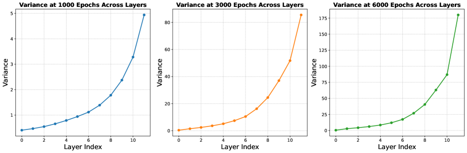![Refer to caption](https://arxiv.org/html/2502.05795v5/x11.png)Figure 9:Variance growth across layers in LLaMA\-130M with Pre\-LN\.Each subplot shows the variance at different training stages \(1000, 3000, and 6000 epochs\)\. In all cases, the variance follows an exponential growth pattern as depth increases, indicating that deeper layers experience uncontrolled variance amplification regardless of training progress\.Figure[9](https://arxiv.org/html/2502.05795v5#A2.F9)illustrates the layer\-wise variance in LLaMA\-130M with Pre\-LN at 1000, 3000, and 6000 epochs\. Across all stages, variance remains low in shallow layers but grows exponentially in deeper layers, confirming that this issue persists throughout training rather than being a temporary effect\. This highlights the necessity of stabilization techniques like LayerNorm Scaling to control variance and ensure effective deep\-layer learning\.

## Appendix CPerformance Drop of Layer Pruning in Vision–Language Models \(Qwen 2\.5\-VL\)

To examine whether theCurse of Depthalso manifests in vision–language models \(VLMs\), we perform layer–pruning experiments onQwen 2\.5\-VL\-7B\(Baiet al\.,[2025](https://arxiv.org/html/2502.05795v5#bib.bib65)\)\. For both its vision encoder and language decoder, we prune one transformer layer at a time and directly evaluate the pruned model on the MMMU benchmark\(Yueet al\.,[2024](https://arxiv.org/html/2502.05795v5#bib.bib64)\)\. Figure[10](https://arxiv.org/html/2502.05795v5#A3.F10)presents the resulting performance drops\.

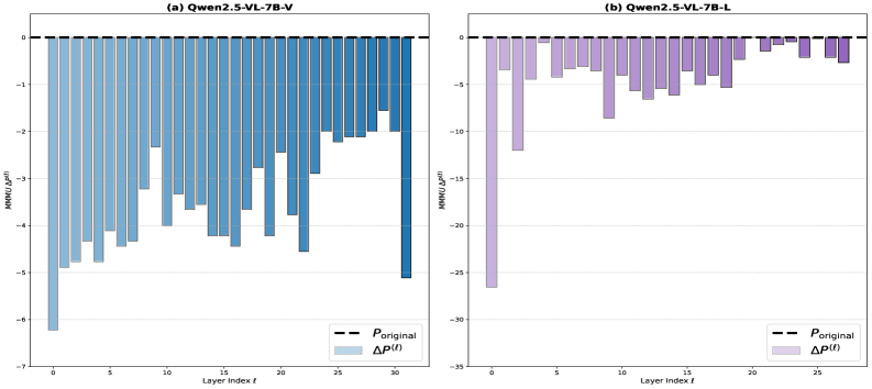![Refer to caption](https://arxiv.org/html/2502.05795v5/x12.png)Figure 10:Performance drop of layer pruning on Qwen 2\.5\-VL\-7B\. \(a\) Vision branch shows relatively uniform sensitivity across layers\. \(b\) Language branch exhibits a clearCurse of Depth: deeper layers contribute much less than early ones\.We observe that thelanguage branchclearly suffers from the Curse of Depth, whereas thevision branchremains uniformly important\. This suggests that the phenomenon is more pronounced in autoregressive language components of VLMs and may not directly transfer to vision encoders\. A detailed modality–specific theoretical account is left to future work and community discussion\.

## Appendix DLimitations

While this work offers a comprehensive analysis of the Curse of Depth in LLMs and proposes LayerNorm Scaling as an effective remedy, several limitations remain:

##### Scope of Architectures\.

Our study primarily focuses on Transformer\-based LLMs using Pre\-LN\. Although Pre\-LN dominates modern architectures, our theoretical study does not cover models employing alternative normalization strategies \(e\.g\., Post\-LN only\(Duet al\.,[2021](https://arxiv.org/html/2502.05795v5#bib.bib8)\), normalization\-free architectures\(Zhuet al\.,[2025a](https://arxiv.org/html/2502.05795v5#bib.bib7)\)\) or emerging paradigms such as mixture\-of\-experts or structured sparsity\-based models\.

##### Task Coverage\.

Most empirical evaluations, including pruning and angular distance analyses, were conducted using general\-purpose benchmarks like MMLU\. While these tasks reflect broad model capabilities, domain\-specific or long\-context reasoning tasks may reveal different dynamics in deep layer contributions, which we leave for future work\.

##### Fine\-grained Representation Quality\.

While LNS improves angular distance and performance sensitivity across layers, a deeper analysis of what types of information are represented or lost in deeper layers remains unexamined\. For example, whether LNS helps preserve syntactic, semantic, or factual knowledge across depth is unclear\.