Starting a new blog post series to better understand modern RL algorithms from the ground up.

Part 1 covers the classic REINFORCE estimator: deriving unbiased policy gradients without differentiating through the environment, and analyzing its variance:

https://t.co/RZ6PrIIfL4

Policy Gradients Part 1: The REINFORCE Estimator

Source: https://fa.bianp.net/blog/2026/policy-gradient/ I have a dirty secret. Well, I actually have many. But one of them is that I never understood the basic algorithms behind reinforcement learning. So I plan to remedy this with a series of blog posts, where I will cover some of the basic RL algorithms, from REINFORCE to the frontier.

Here’s the first one, where I cover one of the oldest practical gradient estimators for reinforcement learning, the REINFORCE estimator, and show how it can get away without differentiating through the environment.

Setup

This is the notation I’ll follow throughout the series. An agent interacts with an environment by observing states s \\in \\mathcal\{S\}, taking actions a \\in \\mathcal\{A\}, receiving rewards r\(s, a\) \\in \\RR, and transitioning to a new state s' according to the environment’s transition probability distribution \{\\color\{colordynamics\}p\(s' \| s, a\)\}. We write the initial state distribution over s\_0 \\in \\mathcal\{S\} simply as \{\\color\{colordynamics\}p\(s\_0\)\}.

The agent’s behavior is determined by apolicy\{\\color\{colorpolicy\}\\pi\_\\theta\(a \| s\)\}, which maps states to distributions over actions. This policy has parameters \\theta \\in \\RR^d, and we’d like to find parameters that maximize the expected return: \begin{equation}\label{eq:objective} J(\theta) \defas \EE_{\tau \sim {\color{colorpolicy}\pi_\theta}}\left[ {\color{colorreturn}R(\tau)} \right] = \int p(\tau | \theta) \, {\color{colorreturn}R(\tau)} \, \dif\tau\,, \end{equation} where \{\\color\{colorreturn\}R\(\\tau\)\} = \\sum\_\{t=0\}^\{T\-1\} r\(s\_t, a\_t\) is the return of a trajectory \\tau = \(s\_0, a\_0, s\_1, a\_1, \\ldots, s\_\{T\-1\}, a\_\{T\-1\}, s\_T\), T is the trajectory length or horizon (which may be fixed or determined by the environment when reaching a terminal state), and p\(\\tau \| \\theta\) is the probability of observing that trajectory \\tau under policy \{\\color\{colorpolicy\}\\pi\_\\theta\}. For simplicity, we focus here on undiscounted finite-horizon returns, though all derivations extend directly to discounted returns R\(\\tau\) = \\sum\_\{t=0\}^\{T\-1\} \\gamma^t r\(s\_t, a\_t\) with discount factor \\gamma \\in \[0, 1\). Throughout, we color-code the key quantities: \{\\color\{colorpolicy\}\\text\{green\}\} for the policy, \{\\color\{colorreturn\}\\text\{orange\}\} for the return, and \{\\color\{colordynamics\}\\text\{purple\}\} for the environment dynamics.

When Things go South

Suppose we want to maximize the expected return J\(\\theta\) using gradient ascent. Writing out the gradient of the expected return gives: \begin{equation}\label{eq:naive_grad} \nabla_\theta J(\theta) = \nabla_\theta \int p(\tau | \theta) {\color{colorreturn}R(\tau)} \dif\tau = \int \nabla_\theta p(\tau | \theta) {\color{colorreturn}R(\tau)} \dif\tau\,. \end{equation} To evaluate this integral, we need to compute the gradient of the trajectory probability \\nabla\_\\theta p\(\\tau \| \\theta\). Using the chain rule of probability, the probability of a trajectory \\tau under policy \{\\color\{colorpolicy\}\\pi\_\\theta\} is a product of initial state probabilities, policy choices, and environment transitions:\begin{equation}\label{eq:trajectory_prob} p(\tau | \theta) = {\color{colordynamics}p(s_0)} \prod_{t=0}^{T-1} {\color{colorpolicy}\pi_\theta(a_t | s_t)} \, {\color{colordynamics}p(s_{t+1} | s_t, a_t)}\,. \end{equation}

Now we hit a wall. To compute \\nabla\_\\theta p\(\\tau \| \\theta\), we would need to differentiate this product with respect to \\theta. But the product contains the environment’s transition dynamics \{\\color\{colordynamics\}p\(s\_\{t\+1\} \| s\_t, a\_t\)\}, which are typically a black box: a robot arm colliding with an object involves discontinuous contact forces, and a board game advances by discrete rules. In either case, we do not have analytical or differentiable access to the transition function, so we cannot compute \\nabla\_\\theta p\(\\tau \| \\theta\) directly.

The Log-Derivative Trick

To move forward, we turn to a classic identity in stochastic optimization known as thelog-derivative trick(also known as the likelihood-ratio method or score function estimator).For a broader perspective on score functions and their connection to integration by parts and randomized smoothing, seeFrancis Bach’s excellent blog post.For any differentiable probability density p\_\\theta\(x\) \> 0, we have the identity \\nabla\_\\theta p\_\\theta\(x\) = p\_\\theta\(x\) \\, \\nabla\_\\theta \\log p\_\\theta\(x\), which follows from the chain rule: \begin{equation}\label{eq:log_derivative_trick} \nabla_\theta \log p_\theta(x) = \frac{\nabla_\theta p_\theta(x)}{p_\theta(x)}\,. \end{equation}

This identity lets us rewrite the problematic gradient \\nabla\_\\theta p\(\\tau \| \\theta\) in terms of \\nabla\_\\theta \\log p\(\\tau \| \\theta\), converting the integral into an expectation: \begin{align} \nabla_\theta J(\theta) &= \int \left( \nabla_\theta p(\tau | \theta) \right) {\color{colorreturn}R(\tau)} \dif\tau \nonumber \\ &= \int p(\tau | \theta) \nabla_\theta \log p(\tau | \theta) {\color{colorreturn}R(\tau)} \dif\tau \nonumber \\ &= \EE_{\tau \sim {\color{colorpolicy}\pi_\theta}}\left[ {\color{colorreturn}R(\tau)} \nabla_\theta \log p(\tau | \theta) \right]\,. \label{eq:rl_score_sub} \end{align} We have traded the intractable \\nabla\_\\theta p\(\\tau \| \\theta\) for \\nabla\_\\theta \\log p\(\\tau \| \\theta\) inside an expectation. But is this any better?

The World Drops Out

Taking the logarithm of the trajectory probability \\eqref\{eq:trajectory\_prob\} turns the product into a sum: \begin{equation}\label{eq:log_trajectory_prob} \log p(\tau | \theta) = \log {\color{colordynamics}p(s_0)} + \sum_{t=0}^{T-1} \log {\color{colorpolicy}\pi_\theta(a_t | s_t)} + \sum_{t=0}^{T-1} \log {\color{colordynamics}p(s_{t+1} | s_t, a_t)}\,. \end{equation} This is crucial: turning a multiplicative structure into an additive one makes differentiation much easier. Taking the gradient with respect to \\theta yields: \begin{equation}\label{eq:grad_log_trajectory} \nabla_\theta \log p(\tau | \theta) = \underbrace{\nabla_\theta \log {\color{colordynamics}p(s_0)}}_{= \, 0} + \sum_{t=0}^{T-1} \nabla_\theta \log {\color{colorpolicy}\pi_\theta(a_t | s_t)} + \underbrace{\sum_{t=0}^{T-1} \nabla_\theta \log {\color{colordynamics}p(s_{t+1} | s_t, a_t)}}_{= \, 0}\,. \end{equation} The environment dynamics \{\\color\{colordynamics\}p\(s\_\{t\+1\} \| s\_t, a\_t\)\} describe the fixed laws of the environment, not the agent’s policy, and so their derivatives with respect to \\theta are identically zero. Likewise, the initial state distribution \{\\color\{colordynamics\}p\(s\_0\)\} does not depend on \\theta. The unknown environment dynamics drop out entirely, leaving only our differentiable policy: \begin{equation}\label{eq:grad_log_simplified} \nabla_\theta \log p(\tau | \theta) = \sum_{t=0}^{T-1} \nabla_\theta \log {\color{colorpolicy}\pi_\theta(a_t | s_t)} \,. \end{equation}

Substituting \\eqref\{eq:grad\_log\_simplified\} back into \\eqref\{eq:rl\_score\_sub\} gives our fundamental result, the REINFORCE estimator:Pronounced as it’s written, but shouting.

Let \\hat\{g\}\(\\tau\) be the REINFORCE estimator for a trajectory \\tau, defined as: \begin{equation}\label{eq:reinforce} \hat{g}(\tau) = \left(\sum_{t=0}^{T-1} \nabla_\theta \log {\color{colorpolicy}\pi_\theta(a_t | s_t)}\right) {\color{colorreturn}R(\tau)}\,. \end{equation} This is an unbiased estimator of the expected return gradient, that is, \begin{equation}\label{eq:reinforce_expectation} \EE_{\tau \sim {\color{colorpolicy}\pi_\theta}} [\hat{g}(\tau)] = \nabla_\theta J(\theta)\,. \end{equation} This allows us to optimize expected return by sampling trajectories from the environment, without needing to differentiate through its transition dynamics.

TheREINFORCEgradient estimator is commonly attributed to Williams (1992),Fun historical detail:REINFORCEis actually a backronym coined by Williams forREwardIncrement =NonnegativeFactor ×OffsetReinforcement ×CharacteristicEligibility, referring to the structure of the update rule.although the log-derivative trick was known well before that. In optimal control and simulation optimization, this general paradigm of directly parameterizing the control law is known asapproximation in policy space, and the resulting estimator is referred to as thelikelihood ratio method.For a comprehensive exposition of approximation in policy space and likelihood ratio gradient methods, see Chapter 5 of Bertsekas (2019).

Notice what has happened. The gradient \\nabla\_\\theta J\(\\theta\) is expressed as the expected value of the estimator \\hat\{g\}\(\\tau\), which involves only the policy’s log-probabilities and the return. The transition dynamics \{\\color\{colordynamics\}p\(s\_\{t\+1\} \| s\_t, a\_t\)\} appear nowhere in the expression. They are implicit: they determinewhichtrajectories are likely when we sample \\tau \\sim \{\\color\{colorpolicy\}\\pi\_\\theta\}, but we never need to know their functional form or differentiate through them. This is the key insight:the log-derivative trick converts “differentiate the distribution” into “evaluate a score function under the distribution”.

Variance

An unbiased estimator is a good start, but that’s still far from practical. Ideally, this estimator should havelow variance. Under assumptions, we can show that the variance of the REINFORCE gradient estimator is bounded as O\(T^3\), and scales as \\Theta\(T^3\) whenever the expected per-step reward has a non-zero mean.

We’ll make the following assumptions. First, per-step rewards are bounded by a constant r\_\{\\max\}, that is, \|r\(s\_t, a\_t\)\| \\le r\_\{\\max\} for all t. Second, the second moment of the per-step score is bounded, i.e., \\EE\[\\\|\\nabla\_\\theta \\log \\pi\_\\theta\(a\_t \| s\_t\)\\\|^2\] \\le C for some constant C \> 0 and all t.This assumption holds for standard policies: forsoftmax policies, whenever the logit gradients (network Jacobian) are bounded; forGaussian policies\\mathcal\{N\}\(\\mu\_\\theta\(s\), \\sigma^2 I\), whenever the mean network has bounded gradients and the variance \\sigma^2 is bounded away from zero.

Under the assumptions above, the total variance \\text\{Var\}\(\\hat\{g\}\(\\tau\)\) \\defas \\EE\[\\\|\\hat\{g\}\(\\tau\) \- \\EE\[\\hat\{g\}\(\\tau\)\]\\\|^2\] of the REINFORCE estimator is bounded as: \begin{equation}\label{eq:variance_bound} \text{Var}(\hat{g}(\tau)) \le T^3 r_{\max}^2 C = O(T^3)\,. \end{equation}

Show proof

To derive this bound, let’s write the estimator as a product: \\hat\{g\}\(\\tau\) = S\(\\tau\) \\cdot \{\{\\color\{colorreturn\}R\(\\tau\)\}\}, where S\(\\tau\) = \\sum\_\{t=0\}^\{T\-1\} \\nabla\_\\theta \\log \{\\color\{colorpolicy\}\\pi\_\\theta\(a\_t \| s\_t\)\} is the trajectory score. Using the definition of total variance \\text\{Var\}\(\\hat\{g\}\) \\defas \\EE\[\\\|\\hat\{g\} \- \\EE\[\\hat\{g\}\]\\\|^2\] = \\EE\[\\\|\\hat\{g\}\\\|^2\] \- \\\|\\EE\[\\hat\{g\}\]\\\|^2, we have: \begin{equation} \text{Var}(\hat{g}) = \EE[\|S(\tau)\|^2 \, {{\color{colorreturn}R(\tau)}}^2] - \|\nabla_\theta J(\theta)\|^2 \leq \EE[\|S(\tau)\|^2 \, {{\color{colorreturn}R(\tau)}}^2]\,. \end{equation} Since the subtracted term \\\|\\nabla\_\\theta J\(\\theta\)\\\|^2 is non-negative, dropping it gives an upper bound on the variance. Let’s now bound each of the two terms in the remaining expectation.

**1️⃣ The score \\\|S\(\\tau\)\\\|^2 scales as O\(T\).**The score S\(\\tau\) = \\sum\_\{t=0\}^\{T\-1\} \\nabla\_\\theta \\log \{\\color\{colorpolicy\}\\pi\_\\theta\(a\_t \| s\_t\)\} is a sum of T per-step score vectors X\_t \\defas \\nabla\_\\theta \\log \{\\color\{colorpolicy\}\\pi\_\\theta\(a\_t \| s\_t\)\} \\in \\RR^d. Crucially, conditional on the state s\_t, the expectation of the action score is zero: \begin{align*} \EE_{a_t \sim \pi_\theta(\cdot | s_t)} [X_t \mid s_t] &= \int \left( \nabla_\theta \log \pi_\theta(a_t | s_t) \right) \pi_\theta(a_t | s_t) \dif a_t \\ &\stackrel{\eqref{eq:log_derivative_trick}}{=} \int \nabla_\theta \pi_\theta(a_t | s_t) \dif a_t \\ &= \nabla_\theta \underbrace{\int \pi_\theta(a_t | s_t) \dif a_t}_{=\, 1} = 0\,, \end{align*} where we’ve used the fact that \\pi\_\{\\theta\} is a probability distribution that integrates to 1. Now consider any two time steps t < t'. By the law of total expectation: \begin{equation} \EE[X_t^\top X_{t’}]=\EE\Big[\EE[X_t^\top X_{t’} \mid s_0, a_0, \ldots, s_{t’}]\Big]\,. \end{equation}

Inside the inner expectation, the only remaining randomness is the action a\_\{t'\} (by conditioning, everything up to s\_\{t'\} is fixed). Since t < t', X\_t is fully determined by the conditioning set and can be pulled out of the inner expectation. Furthermore, since X\_\{t'\} depends only on s\_\{t'\} and a\_\{t'\}, and a\_\{t'\} is drawn from \\pi\_\\theta\(\\cdot \\mid s\_\{t'\}\), we have \\EE\[X\_\{t'\} \\mid s\_0, a\_0, \\ldots, s\_\{t'\}\]=\\EE\[X\_\{t'\} \\mid s\_\{t'\}\]=0, giving us: \begin{equation} \EE[X_t^\top X_{t’}]=\EE\Big[X_t^\top \underbrace{\EE[X_{t’} \mid s_{t’}]}_{=\, 0}\Big]=0\,. \end{equation} Therefore, score vectors across different steps are uncorrelated, and all cross-terms vanish when expanding the squared norm: \begin{equation} \EE[\|S(\tau)\|^2]=\EE\left[\left\|\sum_{t=0}^{T-1} X_t\right\|^2\right]=\sum_{t=0}^{T-1} \EE[\|X_t\|^2]\,. \end{equation} Under the bounded score variance assumption (\\EE\[\\\|X\_t\\\|^2\] \\leq C for all t),summing over the T steps yields: \begin{equation} \EE[\|S(\tau)\|^2] \le T C = O(T)\,. \end{equation}

**2️⃣ The return \{\{\\color\{colorreturn\}R\(\\tau\)\}\}^2 scales as O\(T^2\).**Using the bounded rewards assumption (\|r\(s\_t, a\_t\)\| \\leq r\_\{\\max\}), we have \|\{\\color\{colorreturn\}R\(\\tau\)\}\| = \|\\sum\_\{t=0\}^\{T\-1\} r\(s\_t, a\_t\)\| \\leq T r\_\{\\max\}. Squaring this upper bound gives the deterministic bound \{\{\\color\{colorreturn\}R\(\\tau\)\}\}^2 \\le T^2 r\_\{\\max\}^2 = O\(T^2\).

**3️⃣ Putting it together.**Since \|\{\\color\{colorreturn\}R\(\\tau\)\}\| \\le T r\_\{\\max\} holds deterministically for every trajectory \\tau, we can bound \{\{\\color\{colorreturn\}R\(\\tau\)\}\}^2 \\le T^2 r\_\{\\max\}^2 pointwise and factor it out of the expectation: \\text\{Var\}\(\\hat\{g\}\) \\le \\EE\[\\\|S\(\\tau\)\\\|^2 \\, \{\{\\color\{colorreturn\}R\(\\tau\)\}\}^2\] \\le T^2 r\_\{\\max\}^2 \\, \\EE\[\\\|S\(\\tau\)\\\|^2\] \\le T^3 r\_\{\\max\}^2 C = O\(T^3\)\\,, which completes the proof.

To put this result in perspective: a cubic dependency on the horizon T isterrible news. Cubic growth means that if you double the length of your episode (say, from 50 to 100 steps), the variance of your gradient estimates does not just double: it multiplies byeight(2^3 = 8). This makes the estimates incredibly noisy for long horizons.

Empirical Variance Scaling

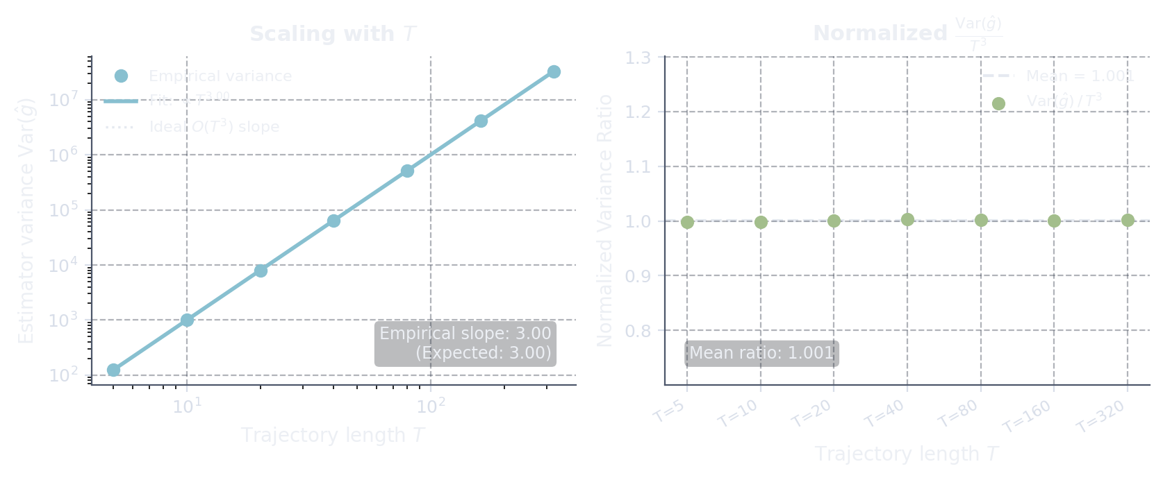
What we derived in the previous section is anupper boundon the variance. For all we know, this bound could be very loose and the real variance scaling factor could be much smaller. To check how the empirical variance scales in practice, we simulate a simple synthetic MDP. Similar toy environments (such as linear-quadratic control systems and contextual bandits) have been used in the literature for isolating and studying gradient variance.

The setup is as follows: at each time step, the agent observes a state s\_t drawn uniformly from \[\-1, 1\]^4 and selects one of \|\\mathcal\{A\}\| = 4 actions according to a softmax linear policy \\pi\_\\theta\(a \| s\) \\propto \\exp\(\\theta\_a^\\top s\), with parameters \\theta drawn from a normal distribution \\mathcal\{N\}\(0, 0\.01^2\). Each step yields a reward r\(s\_t, a\_t\) = 1 \+ 0\.1 \\, \\theta\_\{a\_t\}^\\top s\_t. For each trajectory length T \\in \\\{5, 10, 20, 40, 80, 160, 320\\\}, we estimate \\text\{Var\}\(\\hat\{g\}\) from 30,000 independent trajectories:

• **Left:**Log-log plot of gradient estimator variance \\text\{Var\}\(\\hat\{g\}\) versus trajectory length T, yielding an empirical scaling exponent of 3\.00.
• **Right:**Normalized variance \\frac\{\\text\{Var\}\(\\hat\{g\}\)\}\{T^3\} across various values of T, confirming that the ratio remains tightly around a constant.

Show code to generate plot

"""
Generate a 2-panel figure illustrating REINFORCE variance scaling with trajectory length T: Var(g) = O(T^3).

Setup: Multi-step environment with softmax linear policy.
  - State features: s_t ~ Uniform([-1, 1]^n), with fixed n = 4.
  - Policy: softmax linear pi_theta(a | s) = exp(theta_a^T s) / sum_a' exp(theta_{a'}^T s)
  - Number of actions: |A| = 4 (fixed)
  - theta initialized near zero
  - Reward per step: r(s_t, a_t) = 1 + 0.1 * (theta_{a_t}^T s_t)  (mean reward ~ 1)
  - Score: X_t = (e_{a_t} - pi_t) ⊗ s_t
  - Estimator: g(tau) = R(tau) * S(tau) where S = sum_t X_t
"""

import numpy as np
import matplotlib
matplotlib.use("Agg")
import matplotlib.pyplot as plt
from scipy.special import softmax

# Color palette (Dark theme / Nord palette)
BG_COLOR_FIG = "#1E222A"    # Outer figure background
BG_COLOR_AX = "#252931"     # Subplot panel background
COLOR_TEXT = "#ECEFF4"      # Primary text color
COLOR_MUTED = "#D8DEE9"     # Muted text color
GRID_COLOR = "#3B4252"      # Grid line color
SPINE_COLOR = "#4C566A"     # Border / spine color

COLOR_T = "#88C0D0"         # Nord cyan/blue
COLOR_RATIO = "#A3BE8C"     # Nord green
COLOR_REF = "#E5E9F0"       # Dotted reference line

def simulate_reinforce_gradients(n_samples, T, n_feat, n_actions, rng):
    """
    Simulates trajectories and returns the REINFORCE gradient estimates.
    The policy theta is kept identical using a fixed seed generator.
    """
    theta_rng = np.random.default_rng(0)
    theta = theta_rng.normal(0, 0.01, (n_actions, n_feat))
    d = n_actions * n_feat

    total_scores = np.zeros((n_samples, d))
    total_rewards = np.zeros(n_samples)

    for t in range(T):
        # Sample states: (n_samples, n_feat)
        states = rng.uniform(-1, 1, (n_samples, n_feat))

        # Compute logits and action probabilities: (n_samples, n_actions)
        logits = states @ theta.T
        probs = softmax(logits, axis=1)

        # Sample actions using cumulative probability thresholding
        cum_probs = np.cumsum(probs, axis=1)
        u = rng.uniform(0, 1, n_samples)
        actions = np.sum(cum_probs < u[:, None], axis=1)
        actions = np.clip(actions, 0, n_actions - 1)

        # Compute scores: (e_{a_t} - pi_t) ⊗ s_t
        e_a = np.zeros((n_samples, n_actions))
        e_a[np.arange(n_samples), actions] = 1.0
        diff = e_a - probs

        # Kronecker product: each row of diff ⊗ each row of states
        score_vecs = diff[:, :, None] * states[:, None, :]
        score_vecs = score_vecs.reshape(n_samples, d)
        total_scores += score_vecs

        # Compute step rewards: 1.0 + 0.1 * (theta_a^T s_t)
        theta_a = theta[actions]
        rewards = 1.0 + 0.1 * np.sum(theta_a * states, axis=1)
        total_rewards += rewards

    # REINFORCE estimator: g = R(tau) * S(tau)
    return total_rewards[:, None] * total_scores

def reinforce_variance(n_samples, T, n_feat, n_actions, seed=42):
    """
    Computes the variance of the REINFORCE gradient estimator for trajectory length T.
    """
    rng = np.random.default_rng(seed)
    all_g = simulate_reinforce_gradients(n_samples, T, n_feat, n_actions, rng)
    return np.var(all_g, axis=0).sum()

def run_variance_experiment(T_list, n_samples, n_feat, n_actions):
    """
    Runs the simulation over multiple trajectory lengths T.
    """
    var_vs_T = []
    for T in T_list:
        print(f"Running simulation for T={T}...")
        var_g = reinforce_variance(n_samples, T, n_feat, n_actions, seed=42)
        var_vs_T.append(var_g)
    return np.array(var_vs_T)

def plot_variance_scaling(T_list, var_vs_T, output_path):
    """
    Plots the variance scaling results in a 2-panel figure.
    """
    log_T = np.log(T_list)
    log_var_T = np.log(var_vs_T)
    slope_T, intercept_T = np.polyfit(log_T, log_var_T, 1)
    print(f"\nEmpirical slope wrt T: {slope_T:.4f}")

    ratios = var_vs_T / (T_list ** 3)
    mean_ratio = np.mean(ratios)
    print(f"Mean normalized ratio Var(g)/T^3: {mean_ratio:.4f}")

    fig, (ax1, ax2) = plt.subplots(1, 2, figsize=(8.5, 3.6))

    for ax in (ax1, ax2):
        ax.set_facecolor("none")
        ax.spines["top"].set_visible(False)
        ax.spines["right"].set_visible(False)
        ax.spines["left"].set_color(SPINE_COLOR)
        ax.spines["bottom"].set_color(SPINE_COLOR)
        ax.tick_params(colors=COLOR_MUTED, labelsize=9)
        ax.grid(True, linestyle="--", alpha=0.4, color=GRID_COLOR)

    fig.patch.set_facecolor("none")

    # --- Panel 1: Var vs T ---
    ax1.loglog(T_list, var_vs_T, "o", color=COLOR_T, ms=6, label="Empirical variance", zorder=3)
    fit_T = np.exp(intercept_T) * (T_list ** slope_T)
    ax1.loglog(T_list, fit_T, "-", color=COLOR_T, lw=2, label=f"Fit: $\\propto T^{{{slope_T:.2f}}}$", zorder=2)
    # Reference line T^3
    ref_T = var_vs_T[0] * (T_list / T_list[0])**3
    ax1.loglog(T_list, ref_T, ":", color=COLOR_REF, lw=1.2, label=r"Ideal $O(T^3)$ slope", zorder=1)

    ax1.set_xlabel("Trajectory length $T$", fontsize=10, color=COLOR_TEXT)
    ax1.set_ylabel(r"Estimator variance $\mathrm{Var}(\hat{g})$", fontsize=10, color=COLOR_TEXT)
    ax1.set_title(r"Scaling with $T$", fontsize=11, fontweight="bold", color=COLOR_TEXT, pad=8)
    leg1 = ax1.legend(fontsize=8, loc="upper left", frameon=False)
    plt.setp(leg1.get_texts(), color=COLOR_TEXT)

    ax1.text(0.95, 0.08, f"Empirical slope: {slope_T:.2f}\n(Expected: 3.00)",
             transform=ax1.transAxes, fontsize=8.5, color=COLOR_TEXT, ha="right",
             bbox=dict(boxstyle="round,pad=0.3", facecolor="#1E222A", alpha=0.3, edgecolor="none"))

    # --- Panel 2: Normalized ratio Var(g) / T^3 ---
    x_pos = np.arange(len(T_list))
    ax2.axhline(mean_ratio, color=COLOR_REF, lw=1.5, ls="--", label=f"Mean = {mean_ratio:.3f}", zorder=1)
    ax2.scatter(x_pos, ratios, color=COLOR_RATIO, s=35, zorder=3, label=r"$\mathrm{Var}(\hat{g})\,/\,T^3$")
    ax2.set_xticks(x_pos)
    ax2.set_xticklabels([f"T={t}" for t in T_list], rotation=30, ha="right", fontsize=8)
    ax2.set_ylim(mean_ratio * 0.7, mean_ratio * 1.3)
    ax2.set_xlabel("Trajectory length $T$", fontsize=10, color=COLOR_TEXT)
    ax2.set_ylabel(r"Normalized Variance Ratio", fontsize=10, color=COLOR_TEXT)
    ax2.set_title(r"Normalized $\frac{\mathrm{Var}(\hat{g})}{T^3}$", fontsize=11, fontweight="bold", color=COLOR_TEXT, pad=8)
    leg2 = ax2.legend(fontsize=8, loc="upper right", frameon=False)
    plt.setp(leg2.get_texts(), color=COLOR_TEXT)

    ax2.text(0.05, 0.08, f"Mean ratio: {mean_ratio:.3f}",
             transform=ax2.transAxes, fontsize=8.5, color=COLOR_TEXT, ha="left",
             bbox=dict(boxstyle="round,pad=0.3", facecolor="#1E222A", alpha=0.3, edgecolor="none"))

    plt.tight_layout()
    plt.savefig(output_path, dpi=200, bbox_inches="tight", transparent=True)
    print(f"\nSaved 2-panel figure to {output_path}")

if __name__ == "__main__":
    n_samples = 30000
    n_actions = 4
    n_feat = 4
    T_list = np.array([5, 10, 20, 40, 80, 160, 320])
    output_img_path = "/Users/pedregosa/dev/webpage/content/images/2026/reinforce_variance_scaling.png"

    var_vs_T = run_variance_experiment(T_list, n_samples, n_feat, n_actions)
    plot_variance_scaling(T_list, var_vs_T, output_img_path)

The message here is that the O\(T^3\) upper bound is not wildly pessimistic, but painfully accurate. Fitting a power law on a log-log scale matches the theoretical O\(T^3\) bound with remarkable precision.

Why does the empirical variance scale tightly as \\Theta\(T^3\)? Intuition comes from considering an environment where per-step rewards have a non-zero mean \\mu\_r = \\EE\[r\(s\_t, a\_t\)\] \\neq 0. In that regime, the return is dominated by its mean, \{\\color\{colorreturn\}R\(\\tau\)\} \\approx T \\mu\_r, so the REINFORCE estimator behaves as \\hat\{g\}\(\\tau\) \\approx \(T \\mu\_r\) S\(\\tau\). Squaring T \\mu\_r multiplies the linear \\Theta\(T\) variance of the uncorrelated score sum S\(\\tau\) by T^2 \\mu\_r^2, yielding a variance that scales strictly as \\Theta\(T^3\).

Summary

The central achievement of the REINFORCE algorithm is that it allows us to optimize policies without knowing or differentiating through the environment’s transition dynamics. By applying the log-derivative trick, the product of transition probabilities turns into a sum, and all environment-dependent terms drop out.

However, the price we pay for this model-free elegance is high variance. Specifically, as we derived above, the variance of the REINFORCE estimator scales cubically with the trajectory length (O\(T^3\)). This stems from the combination of a return R\(\\tau\) that grows linearly with T (contributing an O\(T^2\) term when squared) and a sum of score vectors S\(\\tau\) whose variance also grows linearly as O\(T\) due to uncorrelated steps. As a result, even a moderate increase in the episode horizon T leads to a massive explosion in variance, requiring a prohibitively large number of samples to obtain stable gradient estimates.

In the next post we’ll cover some techniques to reduce the variance of this estimator.

Citing

If you find this blog post useful, please consider citing as:

Policy Gradients Part 1: The REINFORCE Estimator, Fabian Pedregosa, 2026

with bibtex entry:

@misc{pedregosa2026policygradient,
  author = {Pedregosa, Fabian},
  title = {Policy Gradients Part 1: The REINFORCE Estimator},
  year = {2026},
  howpublished = {\url{http://fa.bianp.net/blog/2026/policy-gradient/}},
}

References