PPO had a second wave in the LLM era for reasons unanticipated by the original paper - the importance-ratio objective fixes biases from numeric error, async training, and forward pass noise - the clipping objective affects entropy through a mechanism that we didn’t know about at the time of publication (DAPO, https://arxiv.org/abs/2509.26114)

Clip-Low Increases Entropy and Clip-High Decreases Entropy in Reinforcement Learning of Large Language Models

Source: https://arxiv.org/html/2509.26114 Jaesung R. Park1Junsu Kim2Gyeongman Kim3 Jinyoung Jo4Sean Choi5Jaewoong Cho3Ernest K. Ryu1 1Department of Mathematics, UCLA2Department of Mathematical Sciences, Seoul National University3KRAFTON4Department of Linguistics, Stanford University5Department of Computer Science and Engineering, Santa Clara University

Abstract

Reinforcement learning with verifiable rewards (RLVR) has recently emerged as the leading approach for enhancing the reasoning capabilities of large language models (LLMs). However, RLVR is prone to entropy collapse, where the LLM quickly converges to a near-deterministic form, hindering exploration and progress during prolonged RL training. In this work, we reveal that the clipping mechanism in PPO and GRPO induces biases on entropy. Through theoretical and empirical analyses, we show that clip-low increases entropy, while clip-high decreases it. Further, under standard clipping parameters, the effect of clip-high dominates, resulting in an overall entropy reduction even when purely random rewards are provided to the RL algorithm. Our findings highlight an overlooked confounding factor in RLVR: independent of the reward signal, the clipping mechanism influences entropy, which in turn affects the reasoning behavior. Furthermore, our analysis demonstrates that clipping can be deliberately used to control entropy. Specifically, with a more aggressive clip-low value, one can increase entropy, promote exploration, and ultimately prevent entropy collapse in RLVR training.

1Introduction

Reinforcement learning with verifiable rewards (RLVR) has recently emerged as the leading approach for enhancing the reasoning capabilities of large language models (LLMs), especially in the domain of mathematical reasoning(Guo et al.,2025; Lambert et al.,2024; Luong et al.,2024; Yang et al.,2025). However, RLVR is prone to entropy collapse: a phenomenon where the LLM quickly converges to a near-deterministic form, hindering exploration and progress during prolonged RL training(Yu et al.,2025).

Recent studies have reported this effect and continue to debate whether it is an inevitable byproduct of improved performance(Yue et al.,2025; Cui et al.,2025; Wu et al.,2025). A number of works have proposed heuristic interventions to mitigate entropy collapse, such as tuning training hyperparameters(Yu et al.,2025)or explicitly incorporating a KL-divergence loss term(Liu et al.,2025a). Although these approaches can increase policy entropy to some extent, they fall short of providing a mechanistic understanding of why and how entropy evolves during RL training for LLMs.

Contribution.

In this paper, we elucidate this poorly understood entropy dynamics during RL training of LLMs. First, we theoretically analyze a toy setting where the reward israndom, i.e., independent of the policy distribution, and we prove that the clipping mechanism used in PPO(Schulman et al.,2017)or GRPO(Shao et al.,2024)induces biases on entropy. Specifically, the lower clip (‘clip-low’) on negative advantages increases entropy, while the upper clip (‘clip-high’) on positive advantages decreases entropy. Next, we empirically demonstrate that the theoretical results extend to general RLVR settings for mathematical reasoning tasks. By simply tuning the clipping hyperparameters, we can effectively control the entropy dynamics during RLVR, thereby preventing entropy collapse. Moreover, we show that this entropy-controlled training preserves the base model’s exploration capability without compromising its performance, providing a practical tool for stable and prolonged RLVR training.

1.1Related works

Mitigating Entropy collapse in RLVR.

A growing line of work has investigated the entropy collapse phenomenon. DAPO(Yu et al.,2025)argued that the clip-high component in PPO(Schulman et al.,2017)and GRPO(Shao et al.,2024)prevents the ‘exploration tokens’ from being pushed up, accelerating entropy decay. To counter this, they propose ‘clip-higher’, an asymmetric clipping rule that reduces the clip-high events by settingεhigh>εlow\varepsilon_{\mathrm{high}}>\varepsilon_{\mathrm{low}}. ProRL(Liu et al.,2025a)adopts clip-higher and further emphasizes the use of KL divergence loss for stabilizing entropy; they monitor the training process and manually hard reset the optimization states and reference policy for KL divergence term multiple times to enable prolonged RLVR training. Another popular approach is to use reward shaping to promote exploration(Cheng et al.,2025; Gao et al.,2025a), which could be understood largely as methods motivated by conventional reinforcement learning algorithms(Haarnoja et al.,2018; Burda et al.,2019). On the other hand,Cui et al. (2025)conducted an extensive search and provided a different viewpoint that the decreasing entropy during training could actually be understood as a tradeoff with performance, framing entropy collapse as an expected byproduct of training(Deng et al.,2025).

Exploration of LLMs during RLVR.

There is an active debates about whether RLVR elicits genuinely novel reasoning or merely reweights reasoning paths already latent in the base model. On one side, recent analyses contend RLVR largely reshapes sampling distributions over pre-existing chain of thought. These works highlight the degradation of thepass@kmetric during RLVR training(He et al.,2025), and show that post-trained LLMs could underperform the base model whenkkis large(Yue et al.,2025; Wu et al.,2025). On the other hand, conflicting evidence indicates that RLVR can induce capabilities not present in base models(Wen et al.,2025). For example, carefully reshaping the reward function and deploying an enhanced training schedule has shown to be effective in improving exploration during RLVR(Chen et al.,2025; Song et al.,2025). Notably,Liu et al. (2025a)reports cases where RLVR enables solutions to logical tasks that the base model misses even at largekk. Our findings strengthen this latter perspective: we show that deliberately maintaining higher entropy through controlled clipping could improvepass@kwithout degradingmean@k, suggesting that exploration degradation of LLMs is not an inherent limitation of RLVR.

Random reward for RL.

Counterintuitively, recent studies report that RL can improve LLM benchmark scores even with weak, noisy, or entirely random rewards(Wang et al.,2025; Lv et al.,2025; Zhu et al.,2025). This line of research include methods that utilizeentropy minimizationof the policy model(Zhao et al.,2025; Agarwal et al.,2025; Gao et al.,2025b). The work most closely related to ours is(Shao et al.,2025), where the authors train with purely random rewards and observe gains primarily for models in theQwenfamily(Yang et al.,2025). We show that, under the hood, entropy minimization is the consistent driver when training with random rewards, and that this mechanism appears across a broad set of model families rather than beingQwen-specific. This reframes “random-reward improvements” as a predictable consequence of how the clipped RLVR objectives bias policies toward lower-entropy, even when the reward signal provides no information.

1.2Notation and preliminaries

Consider the setup where given a promptxx, an LLMπθ\pi_{\theta}generates a responsey=(y1,…,yT)y=(y_{1},\ldots,y_{T})and a reward functionr​(y)r(y)evaluates it. The objective is to maximize expected reward:

maximize𝜃𝒥​(θ):=𝔼x∼𝒟y∼πθ(⋅∣x)[r​(y)],\begin{array}[]{ll}\underset{\theta}{\mbox{maximize}}&\displaystyle{\mathcal{J}(\theta):=\mathop{\mathbb{E}}_{\begin{subarray}{c}x\sim\mathcal{D}\\ y\sim\pi_{\theta}(\cdot\mid x)\end{subarray}}[r(y)]},\end{array}(1)where𝒟\mathcal{D}denotes the training distribution of prompts.

We formulate this optimization problem into an RL problem. Specifically, consider the MDP with a discrete state space𝒮\mathcal{S}and a finite action space𝒜\mathcal{A}is the finite action space. The state is defined asst=(x,y1,…,yt−1)s_{t}=(x,y_{1},\dots,y_{t-1})and actionata_{t}is the next token to generate, and the transition dynamics is a deterministic one in which the generated token is appended to the state. Finally, the language modelπθ\pi_{\theta}is regarded as the policy, and we refer to this as the reinforcement learning of large language models (RL-LLM) setup.

Given a policy (language model)π\pi, we define its state visitation measure as

dπ​(s)=∑t=0∞ℙ​(st=s)=𝔼​[∑t=0T𝟏st=s],d^{\pi}(s)=\sum_{t=0}^{\infty}\mathbb{P}\big(s_{t}=s\big)=\mathbb{E}\Big[\sum^{T}_{t=0}\mathbf{1}_{s_{t}=s}\Big],where the probability and expectation is with respect tos0=x∼𝒟s_{0}=x\sim\mathcal{D}andat∼π(⋅|st)a_{t}\sim\pi(\cdot\,|\,s_{t})fort=0,1,…t=0,1,\dots.

REINFORCE.

The classical REINFORCE policy gradient estimator(Williams,1992)is given by

∇θ𝒥​(θ)=𝔼x∼𝒟y∼πθ(⋅∣x)[∑t=1T∇θlog⁡πθ​(yt|y<t,x)​At],\nabla_{\theta}\mathcal{J}(\theta)=\mathop{\mathbb{E}}_{\begin{subarray}{c}x\sim\mathcal{D}\\ y\sim\pi_{\theta}(\cdot\mid x)\end{subarray}}\!\Bigg[\sum_{t=1}^{T}\nabla_{\theta}\log\pi_{\theta}\!\big(y_{t}\,|\,y_{<t},x\big)\,A_{t}\Bigg],(2)wherey<t:=(y1,…,yt−1)y_{<t}:=(y_{1},\dots,y_{t-1})andAtA_{t}is an advantage estimate derived from the trajectory-level rewards, such asAt=r​(yT)A_{t}=r(y_{T}).

Although it is possible to perform stochastic gradient descent (ascent) using the stochastic gradients from Equation2(and doing so would avoid the clipping bias that we identify in this work), such an approach is typically less sample-efficient and less stable. Therefore, methods such as PPO(Schulman et al.,2017)and GRPO(Shao et al.,2024)are preferred in the RL-LLM setting.

Group Relative Policy Optimization (GRPO).

GRPO(Shao et al.,2024)is a variant of proximal policy optimization (PPO)(Schulman et al.,2017)adapted for trajectory-level rewards. Given a current policy parameterθold\theta_{\mathrm{old}}, the algorithm samples a promptx∼𝒟x\sim\mathcal{D}andKKresponsesy(1),…,y(K)∼πθold(⋅|x)y^{(1)},\dots,y^{(K)}\sim\pi_{\theta_{\mathrm{old}}}(\cdot\,|\,x). Then, the parameter update toθ\thetais obtained by performing stochastic gradient steps to solve the subproblem

minimize𝜃∑i=1K1T(i)​∑t=1T(i)min⁡(rt(i)​(θ)​At(i),clip⁡(rt(i)​(θ),1−εlow,1+εhigh)​At(i))\begin{array}[]{ll}\underset{\theta}{\mbox{minimize}}&\displaystyle{\sum_{i=1}^{K}\frac{1}{T^{(i)}}\sum^{T^{(i)}}_{t=1}\min\!\left(r_{t}^{(i)}(\theta)\,A_{t}^{(i)},\;\operatorname{clip}\!\big(r_{t}^{(i)}(\theta),\,1-\varepsilon_{\mathrm{low}},\,1+\varepsilon_{\mathrm{high}}\big)\,A_{t}^{(i)}\right)}\end{array}with

rt(i)​(θ)=πθ​(yt(i)|y<t(i),x)πθold​(yt(i)|y<t(i),x),At(i)=r​(y(i))−mean⁡(r​(y(1)),…,r​(y(K)))r_{t}^{(i)}(\theta)=\frac{\pi_{\theta}\big(y_{t}^{(i)}\,\big|\,y_{<t}^{(i)},x\big)}{\pi_{\theta_{\mathrm{old}}}\big(y_{t}^{(i)}\,\big|\,y_{<t}^{(i)},x\big)},\qquad A_{t}^{(i)}=r(y^{(i)})-\operatorname{mean}\big(r(y^{(1)}),\dots,r(y^{(K)})\big)fort=1,…,T(i)t=1,\dots,T^{(i)}andi=1,…,Ki=1,\dots,K.

The clipping mechanism, whose strength is controlled by the hyperparametersεlow\varepsilon_{\mathrm{low}}andεhigh\varepsilon_{\mathrm{high}}, originates from trust-region policy optimization (TRPO)(Schulman et al.,2015). Its purpose is to prevent the optimization for the subproblem from deviating too far from the reference policyπθold\pi_{\theta_{\mathrm{old}}}that generated the responses. Concretely, the importance sampling ratiort(i)​(θ)r_{t}^{(i)}(\theta)is clipped to lie within the range[1−εlow,1+εhigh][1-\varepsilon_{\mathrm{low}},1+\varepsilon_{\mathrm{high}}]depending on the sign ofAt(i)A_{t}^{(i)}. The main thesis of this paper is that the two clipping mechanisms induce biases on entropy.

To be precise, the version of GRPO we present here is more closely aligned with the variant called DAPO(Yu et al.,2025). While the original GRPO formulation(Shao et al.,2024)normalizesAt(i)A_{t}^{(i)}by the standard deviation of the rewards, we follow the prescription of Dr. GRPO(Liu et al.,2025b)and omit this normalization. In addition, whereas the original PPO and GRPO employ a symmetric clipping parameter withεlow=εhigh\varepsilon_{\mathrm{low}}=\varepsilon_{\mathrm{high}}, DAPO introduces asymmetric clipping withεlow<εhigh\varepsilon_{\mathrm{low}}<\varepsilon_{\mathrm{high}}.

Policy entropy.

For any statests_{t}, the token-level (state-conditional) Shannon entropy of the policyπθ\pi_{\theta}is defined as

ℋ​(πθ|st)=−∑a∈𝒜πθ​(a|st)​log⁡πθ​(a|st),\mathcal{H}(\pi_{\theta}\,|\,s_{t})=-\sum_{a\in\mathcal{A}}\pi_{\theta}(a\,|\,s_{t})\log\pi_{\theta}(a\,|\,s_{t}),(3)where𝒜\mathcal{A}(note,|𝒜|<∞|\mathcal{A}|<\infty) is the LLM vocabulary. In practice, we report the average token entropy over responses, evaluated over states encountered under the old policy distributionπθ\pi_{\theta}. For a minibatch of sizeNN, we estimate the entropy with the following formula

ℋ^​(πθ)=−1N​∑i=1N[1T(i)​∑t=1T(i)ℋ​(πθ|st(i))].\hat{\mathcal{H}}(\pi_{\theta})=-\frac{1}{N}\sum_{i=1}^{N}\Bigg[\frac{1}{T^{(i)}}\sum_{t=1}^{T^{(i)}}\mathcal{H}(\pi_{\theta}\,|\,s_{t}^{(i)})\Bigg].(4)

2Theoretical analysis of clipping with random rewards

Following the formulation ofShao et al. (2025), we consider the setting ofrandom rewardsfor the sake of theoretical analysis and scientific inquiry. Specifically, the random rewards are assumed to be statistically independent of both the prompt and the response generated by the LLM, and to have a symmetric distribution (e.g., a reward that takes values0and11with equal probability is symmetric about1/21/2), which in turn leads to GRPO-style advantage estimates having a zero-mean, symmetric distribution.

By construction, such random rewards and the corresponding advantage estimates computed from them contain no learning signal. Indeed, the associated REINFORCE-type policy gradient estimator has zero expectation:

𝔼x∼𝒟yt∼πθ(⋅|y<t,x)A[∑t=1T∇θlog⁡πθ​(yt|y<t)​A]=𝔼x∼𝒟yt∼πθ(⋅|y<t,x)[∑t=1T∇θlog⁡πθ​(yt|y<t)]​𝔼​[A]=0.\displaystyle\mathop{\mathbb{E}}_{\begin{subarray}{c}x\sim\mathcal{D}\\ y_{t}\sim\pi_{\theta}(\cdot|y_{<t},x)\\ A\end{subarray}}\left[\sum_{t=1}^{T}\nabla_{\theta}\log\pi_{\theta}(y_{t}\,|\,y_{<t})A\right]=\mathop{\mathbb{E}}_{\begin{subarray}{c}x\sim\mathcal{D}\\ y_{t}\sim\pi_{\theta}(\cdot|y_{<t},x)\end{subarray}}\left[\sum_{t=1}^{T}\nabla_{\theta}\log\pi_{\theta}(y_{t}\,|\,y_{<t})\right]\mathbb{E}[A]=0.However, GRPO and its variants crucially employ a clipping mechanism, and in this section, we show that this clipping mechanism induces biases on entropy.

2.1Setup for the theoretical analysis

Consider the objective function of the GRPO subproblem:

𝒥​(π;πold)=𝔼x∼𝒟y∼πold(⋅|x)A[1T​∑t=1Tmin⁡(π​(yt|y<t,x)πold​(yt|y<t,x)​A,clip⁡(π​(yt|y<t,x)πold​(yt|y<t,x),1−εlow,1+εhigh)​A)].\mathcal{J}(\pi;\pi_{\mathrm{old}})=\!\!\!\!\!\!\mathop{\mathbb{E}}_{\begin{subarray}{c}x\sim\mathcal{D}\\ y\sim\pi_{\mathrm{old}}(\cdot\,|\,x)\\ A\end{subarray}}\Bigg[\frac{1}{T}\sum^{T}_{t=1}\min\!\left(\tfrac{\pi(y_{t}\,|\,y_{<t},x)}{\pi_{\mathrm{old}}(y_{t}\,|\,y_{<t},x)}\,A,\;\operatorname{clip}\!\big(\tfrac{\pi(y_{t}\,|\,y_{<t},x)}{\pi_{\mathrm{old}}(y_{t}\,|\,y_{<t},x)},\,1-\varepsilon_{\mathrm{low}},\,1+\varepsilon_{\mathrm{high}}\big)\,A\right)\Bigg].We assume the advantageAAis independent of ofxxandyyand satisfies

𝔼​[A]=0,ℙ​(A>0)=ℙ​(A<0)=ν,𝔼​[A​|A>​0]=μ.\mathbb{E}[A]=0,\quad\mathbb{P}(A>0)=\mathbb{P}(A<0)=\nu,\quad\mathbb{E}[A\,|\,A>0]=\mu. The actual GRPO algorithm performs a limited number of optimization steps on the objective𝒥\mathcal{J}, typically using AdamW, which is difficult to model and analyze directly. For the sake of analytical tractability, we assume the use of full batch gradients and consider two simplified formulations: the policy gradient and natural policy gradient algorithms applied to𝒥\mathcal{J}. Namely, the first algorithm is the policy gradient algorithm

θk+1=θk+η​∇θ𝒥​(πθk;πold),\theta_{k+1}=\theta_{k}+\eta\nabla_{\theta}\mathcal{J}(\pi_{\theta_{k}};\pi_{\mathrm{old}}),(5)whereπold\pi_{\mathrm{old}}is an older version ofπθk\pi_{\theta_{k}}that is updated by the outer loop of GRPO andπθ\pi_{\theta}is parameterized as a tabular softmax policy

πθ​(a|s)=exp⁡(θs,a)∑a′∈𝒜exp⁡(θs,a′)for​s∈𝒮,a∈𝒜\pi_{\theta}(a\,|\,s)=\frac{\exp(\theta_{s,a})}{\sum_{a^{\prime}\in\mathcal{A}}\exp(\theta_{s,a^{\prime}})}\qquad\text{for }s\in\mathcal{S},\,a\in\mathcal{A}with state space𝒮\mathcal{S}, finite action space𝒜\mathcal{A}, and trainable parameterθ∈ℝ|𝒮|×|𝒜|\theta\in\mathbb{R}^{|\mathcal{S}|\times|\mathcal{A}|}. The second algorithm is thenaturalpolicy gradient algorithm(Kakade,2001)

πk+1∝πk∘exp⁡(η​∇π𝒥​(πk;πold)),\pi_{k+1}\propto\pi_{k}\circ\exp\big(\eta\nabla_{\pi}\mathcal{J}(\pi_{k};\pi_{\mathrm{old}})\big),(6)where againπold\pi_{\mathrm{old}}is an older version ofπk\pi_{k}that is updated by the outer loop of GRPO and∘\circdenotes element-wise multiplication. As we will see, our analysis of the two algorithms yields results that differ slightly but are qualitatively aligned. Since the two algorithms are considered models of the true GRPO update, this consistency lends further credibility to the qualitative conclusions drawn from our analysis.

Now, define the following probabilistic events

Xk​(s)\displaystyle X_{k}(s)={event such that​πk​(a|s)πold​(a|s)<1−εlow}\displaystyle=\Big\{\text{event such that }\tfrac{\pi_{k}(a|s)}{\pi_{\mathrm{old}}(a|s)}<1-\varepsilon_{\mathrm{low}}\Big\}=\displaystyle={event such that clip-low happens}\displaystyle\Big\{\text{event such that clip-low happens}\Big\}Yk​(s)\displaystyle Y_{k}(s)={event such that​πk​(a|s)πold​(a|s)>1+εhigh}\displaystyle=\Big\{\text{event such that }\tfrac{\pi_{k}(a|s)}{\pi_{\mathrm{old}}(a|s)}>1+\varepsilon_{\mathrm{high}}\Big\}=\displaystyle={event such that clip-high happens}.\displaystyle\Big\{\text{event such that clip-high happens}\Big\}.Whether eventsXk​(s)X_{k}(s)andYk​(s)Y_{k}(s)hold is determined by the actiona∼πold(⋅|s)a\sim\pi_{\mathrm{old}}(\cdot\,|\,s).

2.2First-order analysis of entropy change

We first present our analysis of the entropy change of the policy gradient algorithm.

Theorem 1.

Consider the setup described in Section2.1and the policy gradient algorithm given by Equation5. Then, the change in entropy at statessadmits the first-order approximation

ℋ​(θk+1|s)−ℋ​(θk|s)=μ​ν​η​dπold​(pk​(𝔼​[Q]−𝔼​[Q|Xk])⏟clip-low contribution−qk​(𝔼​[Q]−𝔼​[Q|Yk])⏟clip-high contribution)+𝒪​(η2)\mathcal{H}(\theta_{k+1}\,|\,s)-\mathcal{H}(\theta_{k}\,|\,s)=\mu\nu\eta\;d^{\pi_{\mathrm{old}}}\big(\underbrace{p_{k}(\mathbb{E}[Q]-\mathbb{E}[Q\,|\,X_{k}])}_{\text{clip-low contribution}}-\underbrace{q_{k}(\mathbb{E}[Q]-\mathbb{E}[Q\,|\,Y_{k}])}_{\text{clip-high contribution}}\big)+\mathcal{O}(\eta^{2})whereQ=πk​(a|s)​(log⁡πk​(a|s)+ℋ​(θk|s))Q=\pi_{k}(a\,|\,s)(\log\pi_{k}(a\,|\,s)+\mathcal{H}(\theta^{k}\,|\,s)),pk=ℙ​(Xk)p_{k}=\mathbb{P}(X_{k}),qk=ℙ​(Yk)q_{k}=\mathbb{P}(Y_{k}),dπo​l​dd^{\pi_{old}}is the state visitation measure, and the expectation𝔼\mathbb{E}is taken with respect toa∼πk(⋅|s)a\sim\pi_{k}(\cdot\,|\,s). To clarify, all the terms on the right-hand side depend onss, and it would be more precise to write them asdπo​l​d​(s)d^{\pi_{old}}(s),Q​(s)Q(s),Xk​(s)X_{k}(s),Yk​(s)Y_{k}(s),pk​(s)p_{k}(s), andqk​(s)q_{k}(s). However, we suppress the dependence onssfor notational simplicity.

We defer the proof to AppendixA.

Theorem1separates the contributions of clip-low and clip-high. Decreasingεl​o​w\varepsilon_{low}leads to a largerpk=ℙ​(Xk)p_{k}=\mathbb{P}(X_{k}), thereby amplifying the clip-low term, and vice-versa for clip-high. Moreover, if either clip-low or clip-high is turned off,pk=0p_{k}=0orqk=0q_{k}=0, and only the other term remains.

If the following condition holds:

𝔼​[Q]−𝔼​[Q|Xk]≥0and𝔼​[Q]−𝔼​[Q|Yk]≥0,\mathbb{E}[Q]-\mathbb{E}[Q\,|\,X_{k}]\geq 0\quad\text{and}\quad\mathbb{E}[Q]-\mathbb{E}[Q\,|\,Y_{k}]\geq 0,(7)then the claim that clip-low increases entropy and clip-high decreases entropy is substantiated. Inequalities7, however, are not guaranteed to hold universally, and counterexamples can be constructed where the condition fails. Nevertheless, we empirically observe that Inequalities7are typically satisfied in practice. In particular, Figure1shows that empirical estimates consistently meet these conditions.

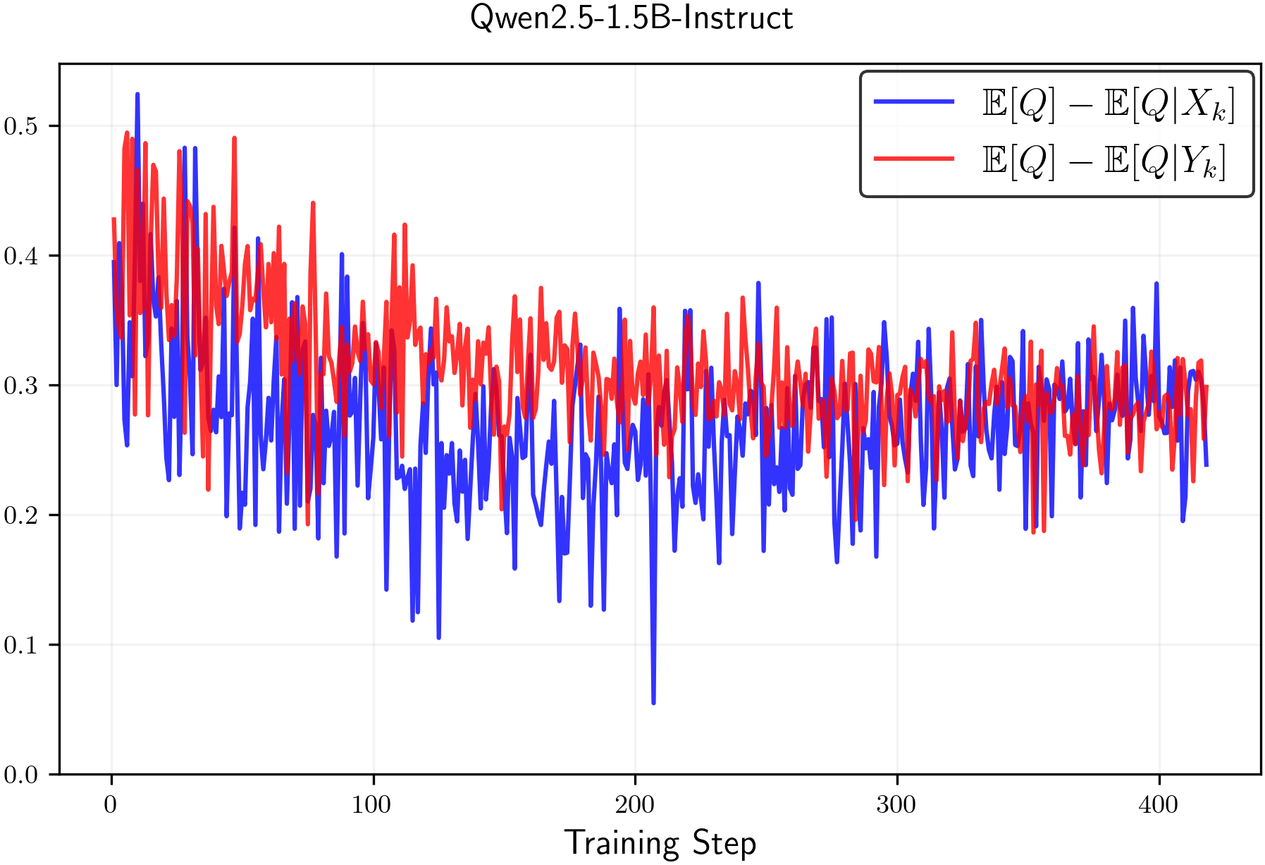
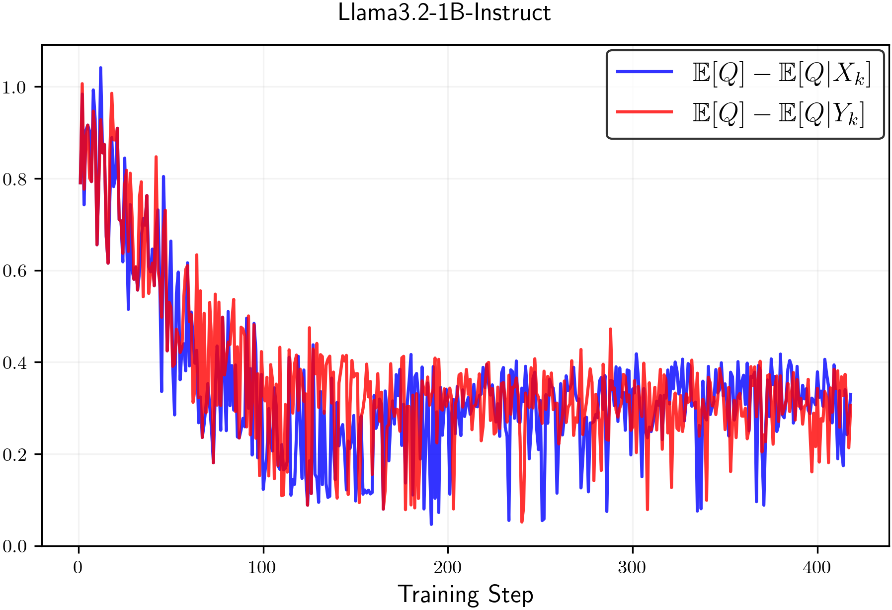
Figure 1:Empirical estimates of𝔼​[Q]−𝔼​[Q|Xk]\mathbb{E}[Q]-\mathbb{E}[Q\,|\,X_{k}]and𝔼​[Q]−𝔼​[Q|Yk]\mathbb{E}[Q]-\mathbb{E}[Q\,|\,Y_{k}]throughout RL training with random rewards for(left)Qwen2.5-1.5B-Instructand(right)Llama3.2-1B-Instruct. We observe that the values are always positive.Next, we present our analysis of the entropy change of thenaturalpolicy gradient algorithm.

Theorem 2.

Consider the setup described in Section2.1and the natural policy gradient algorithm given by Equation6. Then, the change in entropy at statessadmits the first-order approximation

ℋ​(πk+1|s)−ℋ​(πk|s)\displaystyle\mathcal{H}(\pi_{k+1}\,|\,s)-\mathcal{H}(\pi_{k}\,|\,s)=μ​ν​η​dπold​(pk​(𝔼​[−log⁡πk|Xk]−ℋ​(πk|s))⏟clip-low contribution−qk​(𝔼​[−log⁡π|Yk]−ℋ​(πk|s))⏟clip-high contribution)+𝒪​(η2),\displaystyle\qquad=\mu\nu\eta\;d^{\pi_{\mathrm{old}}}\big(\underbrace{p_{k}(\mathbb{E}[-\log\pi_{k}\,|\,X_{k}]-\mathcal{H}(\pi_{k}\,|\,s))}_{\text{clip-low contribution}}-\underbrace{q_{k}(\mathbb{E}[-\log\pi\,|\,Y_{k}]-\mathcal{H}(\pi_{k}\,|\,s))}_{\text{clip-high contribution}}\big)+\mathcal{O}(\eta^{2}),wherepk=ℙ​(Xk)p_{k}=\mathbb{P}(X_{k}),qk=ℙ​(Yk)q_{k}=\mathbb{P}(Y_{k}),dπo​l​dd^{\pi_{old}}is the state visitation measure, and the expectation𝔼\mathbb{E}is taken with respect toa∼πk(⋅|s)a\sim\pi_{k}(\cdot\,|\,s). To clarify, all the terms on the right-hand side depend onss, and it would be more precise to write them asdπo​l​d​(s)d^{\pi_{old}}(s),Xk​(s)X_{k}(s),Yk​(s)Y_{k}(s),pk​(s)p_{k}(s), andqk​(s)q_{k}(s). However, we suppress the dependence onssfor notational simplicity.

We defer the proof to AppendixB.

Theorem2again separates the contributions of clip-low and clip-high. If the following condition holds:

𝔼​[−log⁡πk|Xk]−ℋ​(πk|s)≥0and𝔼​[−log⁡π|Yk]−ℋ​(πk|s)≥0,\mathbb{E}[-\log\pi_{k}\,|\,X_{k}]-\mathcal{H}(\pi_{k}\,|\,s)\geq 0\quad\text{and}\quad\mathbb{E}[-\log\pi\,|\,Y_{k}]-\mathcal{H}(\pi_{k}\,|\,s)\geq 0,(8)then the claim that clip-low increases entropy and clip-high decreases entropy is substantiated. Again, we empirically observe that Inequalities8are typically satisfied in practice. In particular, Figure2shows that empirical estimates consistently meet these conditions.

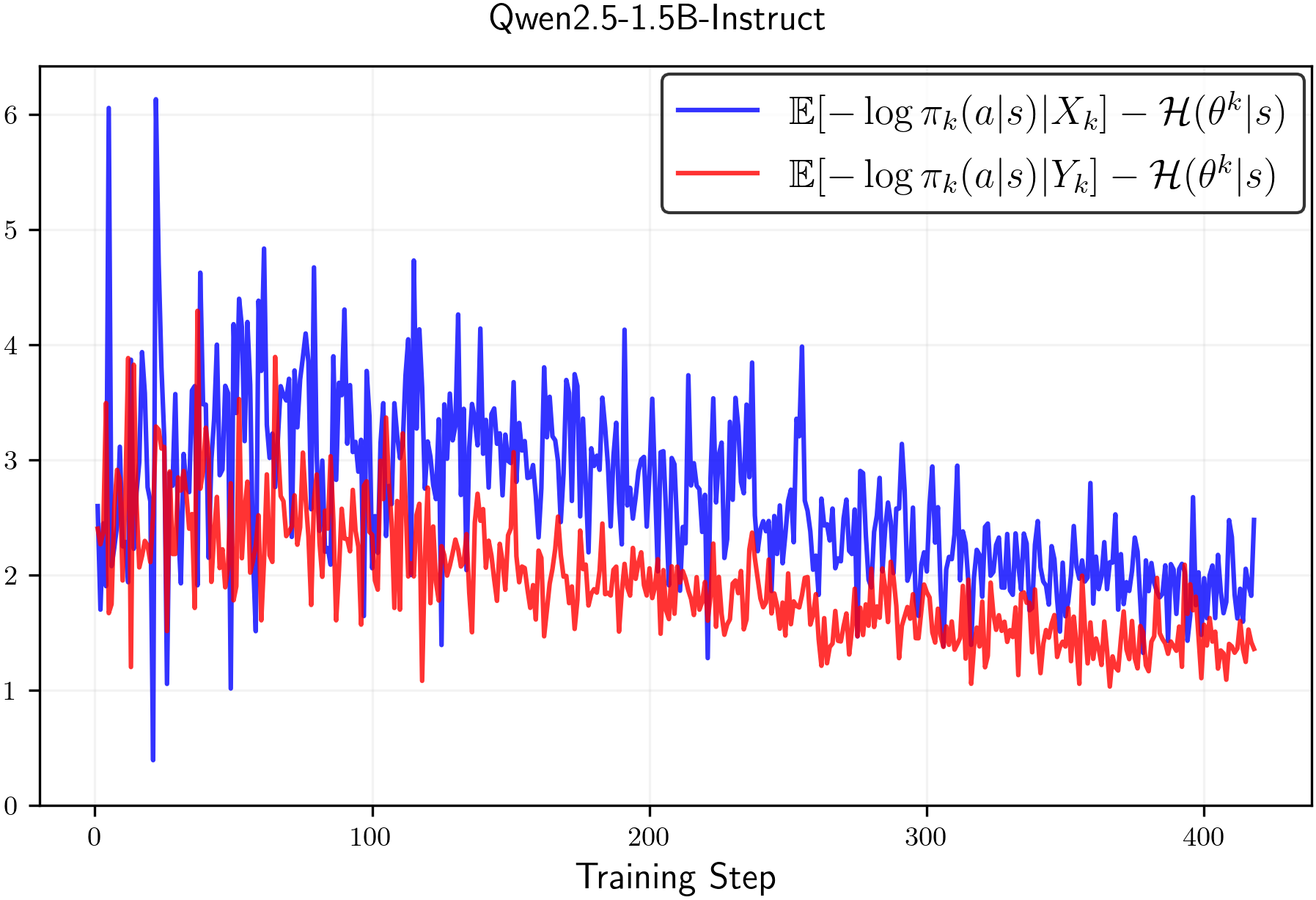
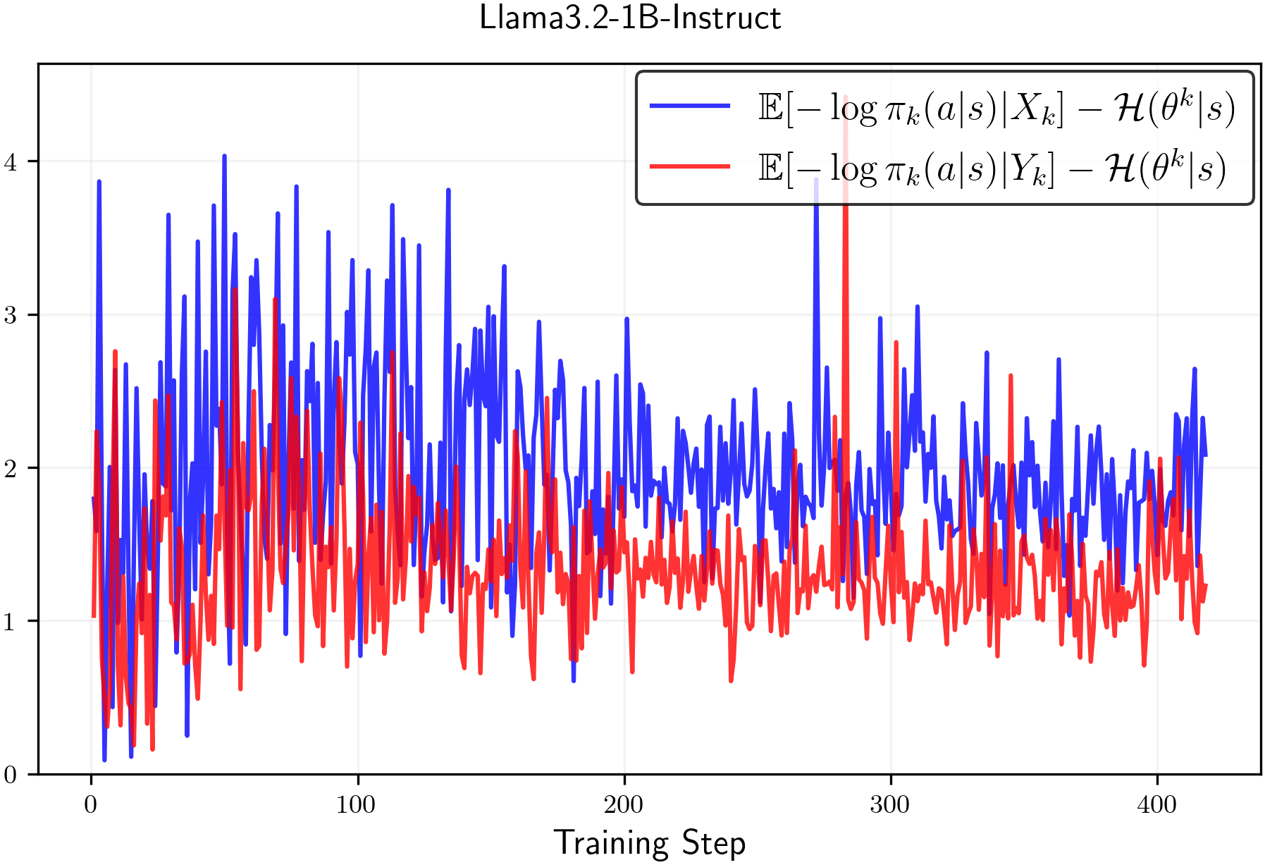
Figure 2:Estimated values of (8) throughout RL training with random rewards averaged over 3 runs.(Left)Qwen2.5-1.5B-Instructand(right)Llama3.2-1.5B-Instruct. We observe that the values are always positive.

2.3Empirical validation

In this section, we present an empirical validation of our theory.

Setting.

We use theverlframework(Sheng et al.,2025)for all experiments. The models are trained with theGSM8Kdataset(Cobbe et al.,2021)but the rewards are randomly drawn from a Bernoulli distribution with0.50.5probability. We use the GRPO algorithm and, following Dr. GRPO(Liu et al.,2025b), we do not normalize rewards by the standard deviation in the advantage calculation. We use theQwen2.5-3B-Instruct(Yang et al.,2024)andLlama3-8B-Instructmodels as our base models. We use a GRPO batch size of512512, and an optimizer batch size of256256. Neither the KL divergence loss nor an explicit entropy loss is applied. For each rollout, we generate88prompts with temperatureT=1T=1. We use theAdamWoptimizer with a constant learning rate of5⋅10−75\cdot 10^{-7}. During validation rollout, we use temperatureT=0.6T=0.6. We defer further implementation details to AppendixC.1.

Figure 3:Change of policy entropy during RL training theQwen2.5-1.5B-Instructmodel with random rewards with different clipping settings. We observe that both clip-high and clip-low influence the entropy, consistent with our theoretical predictions.

Results.

The experimental results are consistent with our theoretical predictions. Figure3shows that decreasing/increasingεlow\varepsilon_{\mathrm{low}}(making clip-low stronger/weaker) increases/decreases entropy, and decreasing/increasingεhigh\varepsilon_{\mathrm{high}}(making clip-high stronger/weaker) decreases/increases entropy.

Moreover, we find that with symmetric clipping parameters (εlow=εhigh=0.2\varepsilon_{\mathrm{low}}=\varepsilon_{\mathrm{high}}=0.2), the effect of clip-high dominates that of clip-low, leading to a reduction in entropy. However, by appropriately decreasingεlow\varepsilon_{\mathrm{low}}(making clip-low stronger), we can counterbalance the competing effects and maintain the entropy level.

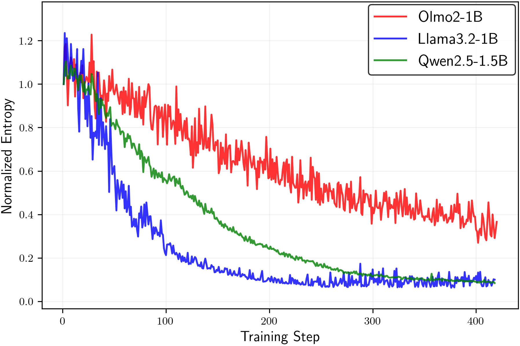
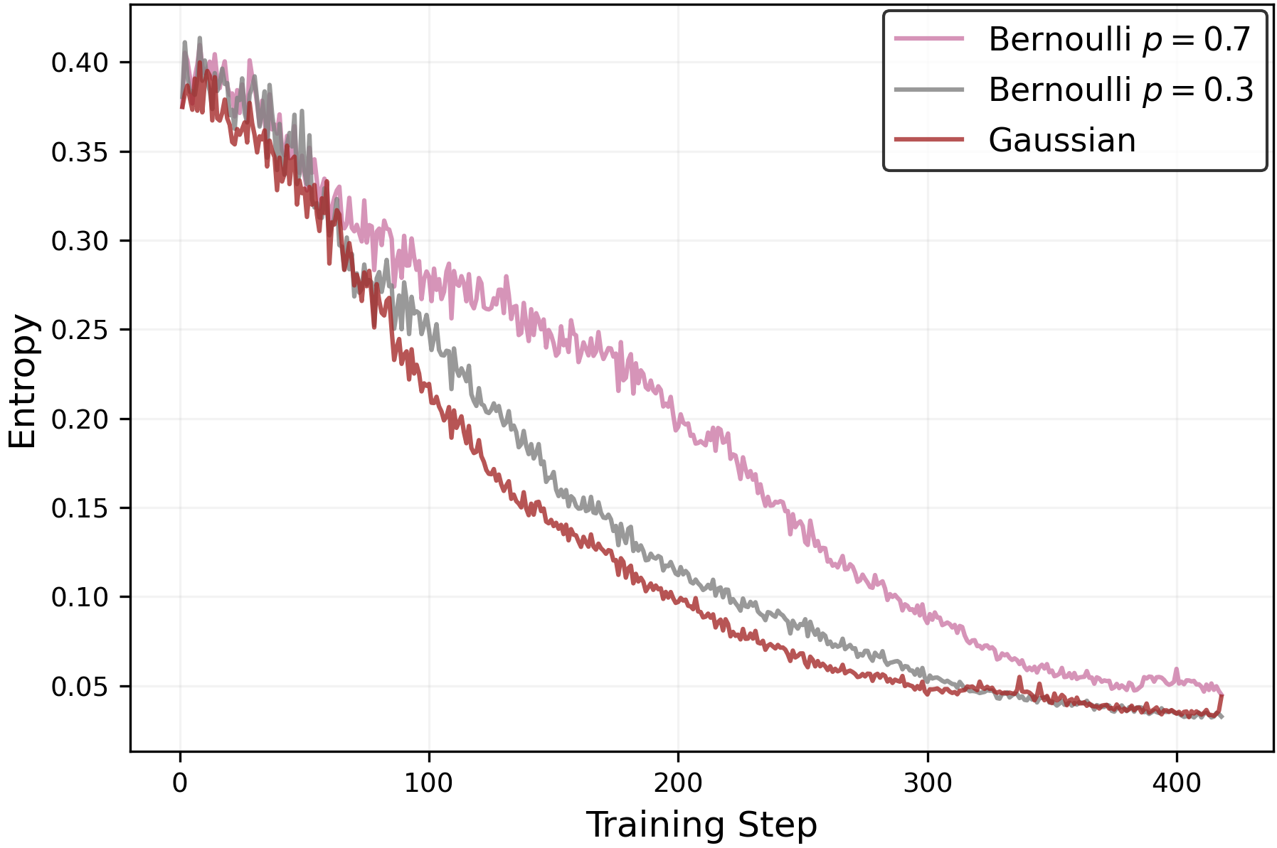
Figure 4:(Left)Entropy change of different base models when trained with random rewards under symmetric clippingεlow=εhigh\varepsilon_{\mathrm{low}}=\varepsilon_{\mathrm{high}}.(Right)Entropy change ofQwen2.5-1.5B-Instructmodel with random rewards sampled from various probability distributions. Details of the experiments are provided in AppendixC.2.

Noisy and spurious rewards reduce entropy.

Prior work has investigated whether RLVR can enhance LLM reasoning even in the presence of noisy rewards(Wang et al.,2025; Lv et al.,2025)or random (spurious) rewards(Shao et al.,2025). In particular,Shao et al. (2025)find that GRPO-based training with clipping yields clear improvements forQwen-based models, but little to no benefit forLlama- orOlmo-based models. By contrast, Figure4shows that training with random rewards consistently reduces policy entropy acrossQwen,Llama, andOlmo. This pattern suggests that the primary effect may be entropy minimization, which in turn influences reasoning behavior as recently suggested in(Agarwal et al.,2025; Gao et al.,2025b).

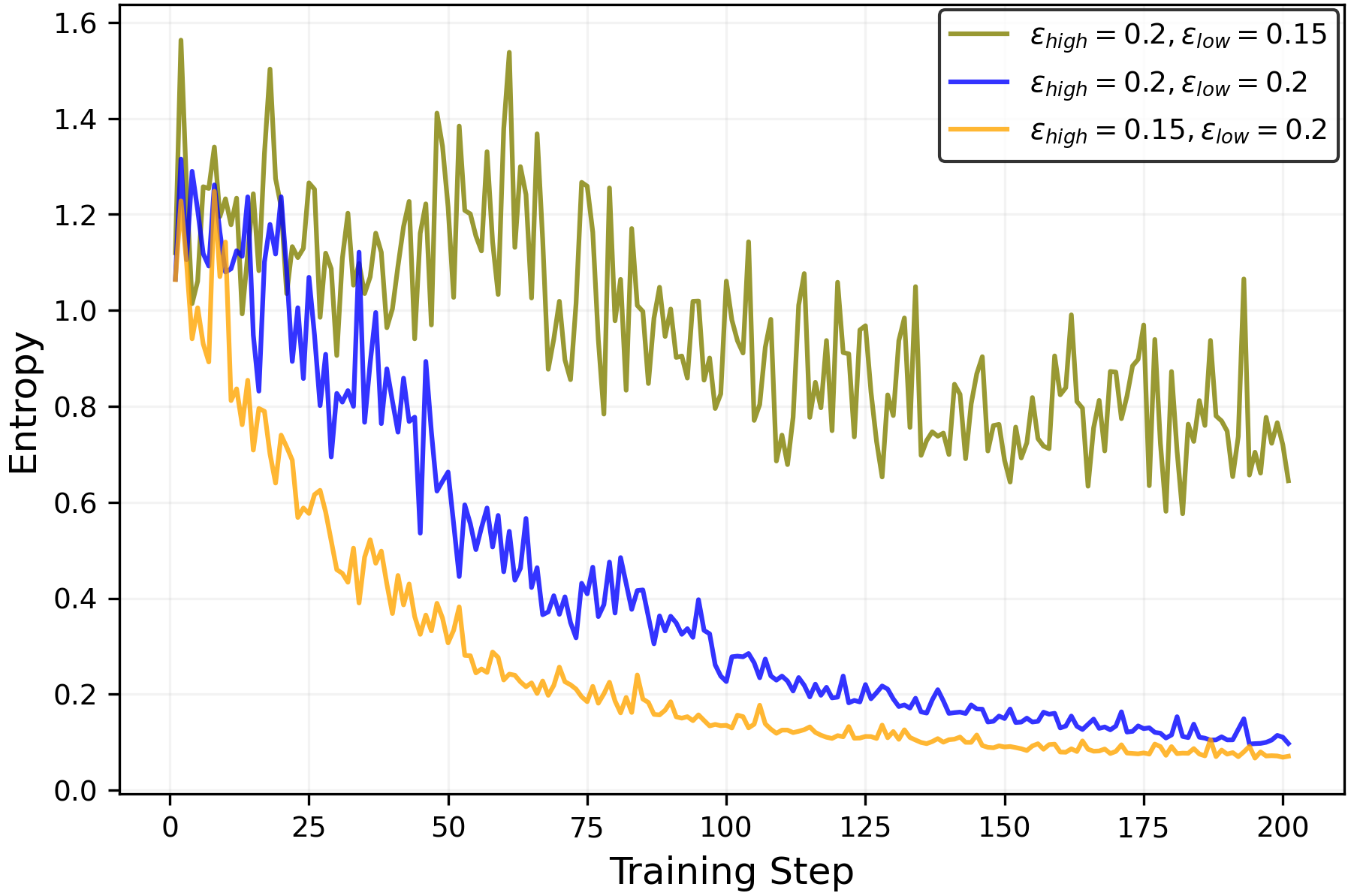
Figure 5:Entropy change during (true reward) RLVR withGSM8KandQwen2.5-3B-Instruct.(Left)Ablating the clipping mechanisms.(Right)Controlling entropy without clip-high. The clip-low valueεlow=0.15\varepsilon_{\mathrm{low}}=0.15balances entropy, preventing entropy collapse and entropy explosion.

3Empirical analysis of clipping with RLVR

In this section, we extend the theoretical insights from the random reward setting of Section2to the general (true reward) RLVR setting through empirical analysis. Our results demonstrate that the clipping parameters,εhigh\varepsilon_{\mathrm{high}}andεlow\varepsilon_{\mathrm{low}}, provide effective control over policy entropy in RLVR for mathematical reasoning tasks. Moreover, such entropy control improves the exploration (as measured bypass@k) while preserving reasoning performance (as measured bymean@8). Specifically, thepass@kmetric measures whether at least one of thekksampled responses yields the correct solution(Chen et al.,2021), whilemean@kreflects the average single-response accuracy (pass@1) across thosekkresponses.

3.1Experimental setup

Again, we use theverlframework(Sheng et al.,2025)for the RL training andGSM8K(Cobbe et al.,2021)and theDAPO-Math-17k(Yu et al.,2025)for the mathematical reasoning training data. ForGSM8K, we useQwen2.5-3B-InstructandLlama3-8B-Instructas base models, and for theDAPO-Math-17kdataset, we useQwen2.5-7B-Instructas the base model. We use the same configurations for the GRPO algorithm as in our random reward experiments of Section2.3. Refer to AppendixC.1for further training details.

(a)Qwen2.5-3B-Instruct

(b)Llama3-8B-Instruct

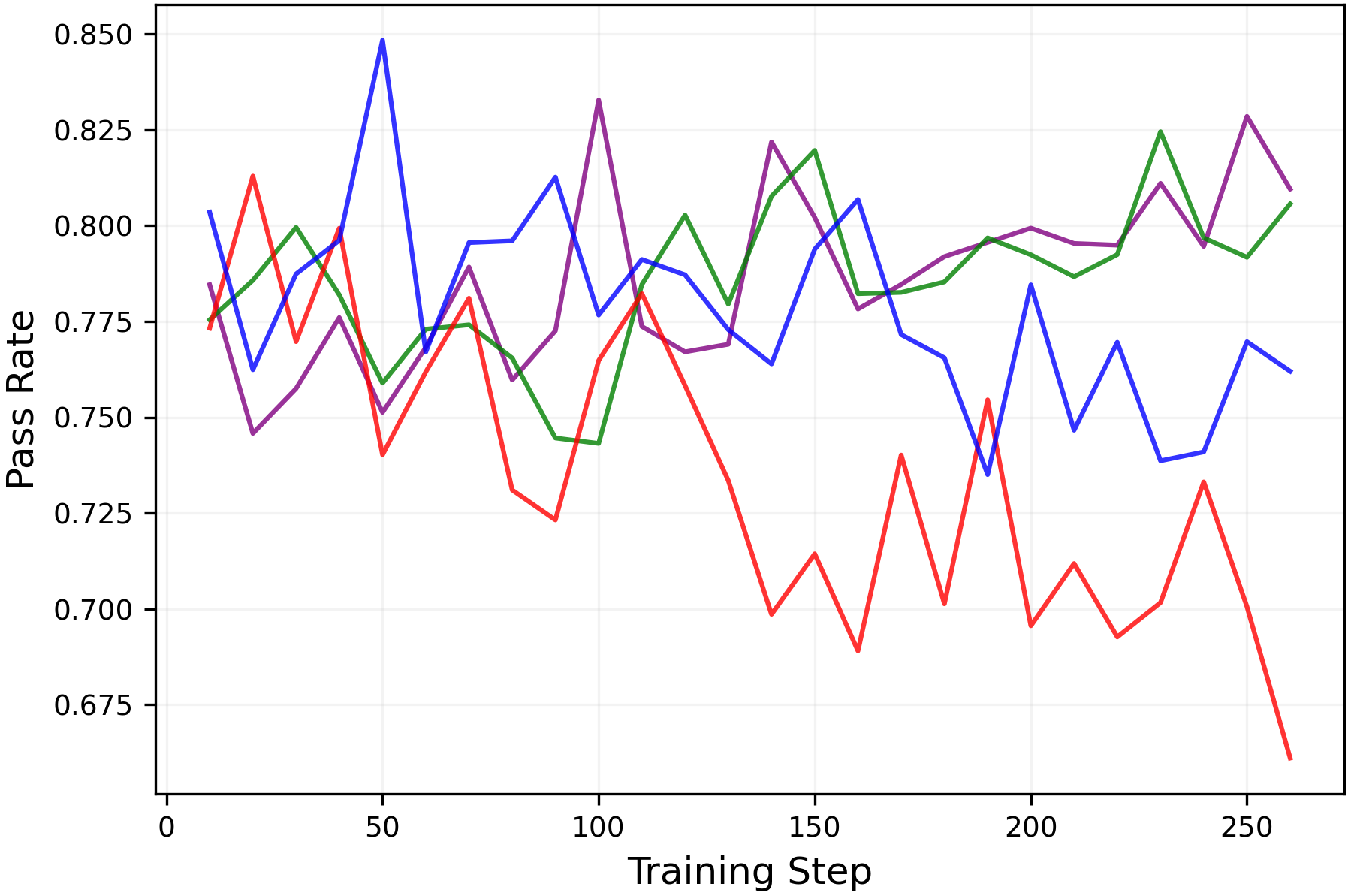
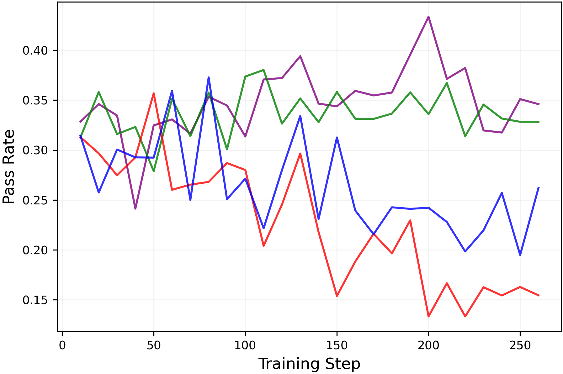
Figure 6:Performance of LLM during RLVR training withGSM8Kdataset measured by the(left)mean@8metric and(right)pass@8metric for(up)Qwen2.5-3B-Instructmodel and(down)Llama3-8B-Instructmodel. While all settings configurations show comparablemean@8performance, training setups with high entropy show higherpass@8performance, implying enhanced exploration.

3.2Experiments: Math reasoning tasks

Clip-high decreases entropy and clip-low increases entropy.

We begin with an ablation study of the clipping mechanisms. Specifically, we disable the clip-low mechanism (by settingεlow=1.0\varepsilon_{\mathrm{low}}=1.0) and the clip-high mechanism (by settingεhigh=∞\varepsilon_{\mathrm{high}}=\infty). As shown in Figure5(left), removing clip-high increases entropy, while removing clip-low decreases it, in qualitative agreement with the theoretical analysis for the random reward setting in Section2.

Entropy control via Clip-Lower

Unlike the random reward setting, RLVR training with true rewards has an entropy-reduction effect, which can be attributed to RLVR’s suppression of incorrect reasoning paths. For example, while the configurationεhigh=∞\varepsilon_{\mathrm{high}}=\infty(clip-high off) andεlow=0.2\varepsilon_{\mathrm{low}}=0.2increased entropy in the random reward setting (Figure3, left), the same configuration leads to reduced entropy in the true reward RLVR setup (Figure5).

To counteract RLVR’s natural entropy reduction, turn off clip-high (εhigh=∞\varepsilon_{\mathrm{high}}=\infty) and adjust the clip-low parameterεlow\varepsilon_{\mathrm{low}}to a smaller value. As shown in Figure5(right), decreasingεlow\varepsilon_{\mathrm{low}}increases entropy during training—sometimes to the extreme of entropy explosion. For this particular setup, we find that the configuration(εhigh=∞,εlow=0.15)(\varepsilon_{\mathrm{high}}=\infty,\varepsilon_{\mathrm{low}}=0.15)achieves a balance, preventing both entropy collapse and entropy explosion.

Entropy control leads to improved exploration.

While RLVR enhances the reasoning performance of LLMs, prior work(Yue et al.,2025; Song et al.,2025)has shown that it also narrows the range of reasoning trajectories the model can explore, also referred to as thereasoning boundary. Consistent with this, Figures6and7shows that training with the standard symmetric clipping parameters (εl​o​w=εh​i​g​h=0.2\varepsilon_{low}=\varepsilon_{high}=0.2) causes thepass@8metric to decline over the course of training.

However, when entropy is controlled through clipping (entropy is shown in Figure5), thepass@8metric is preserved without sacrificing themean@8performance as shown in Figure6. Moreover, Figure7shows that the clipping mechanisms can be tuned to simultaneously improve themean@32andpass@32performances. These results demonstrate that entropy collapse can be avoided through appropriate clipping parameter choices, even without a KL penalty. Moreover, they confirm that this entropy control does genuinely correspond to exploration.

(a)AMC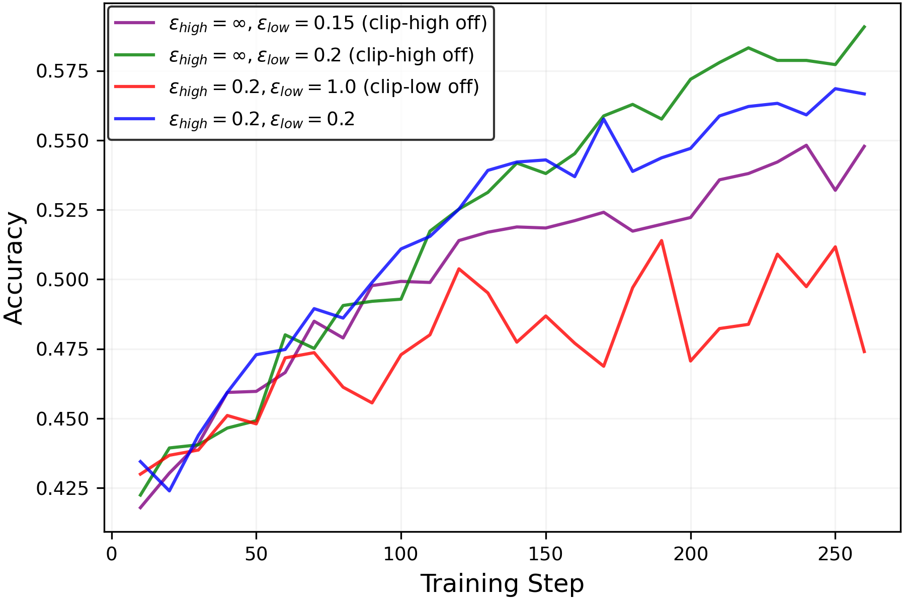

(b)MATH-500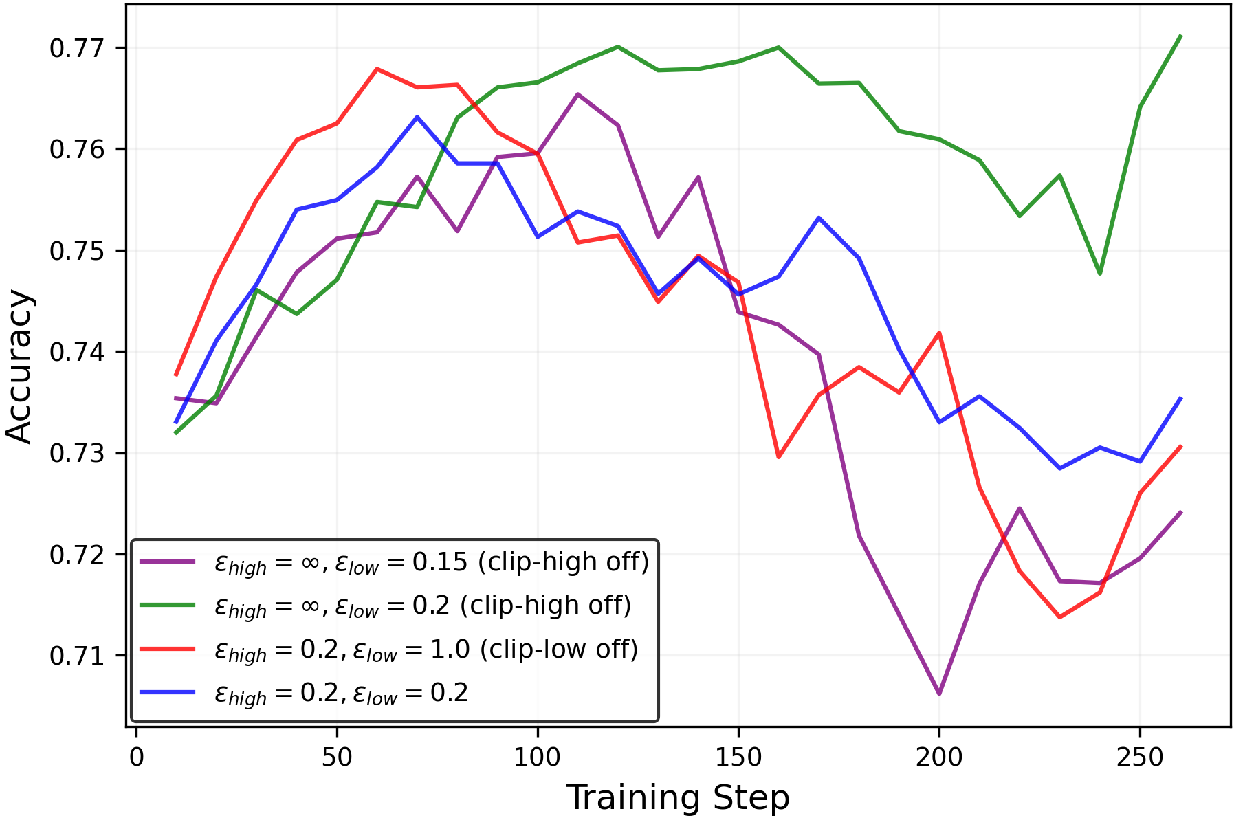

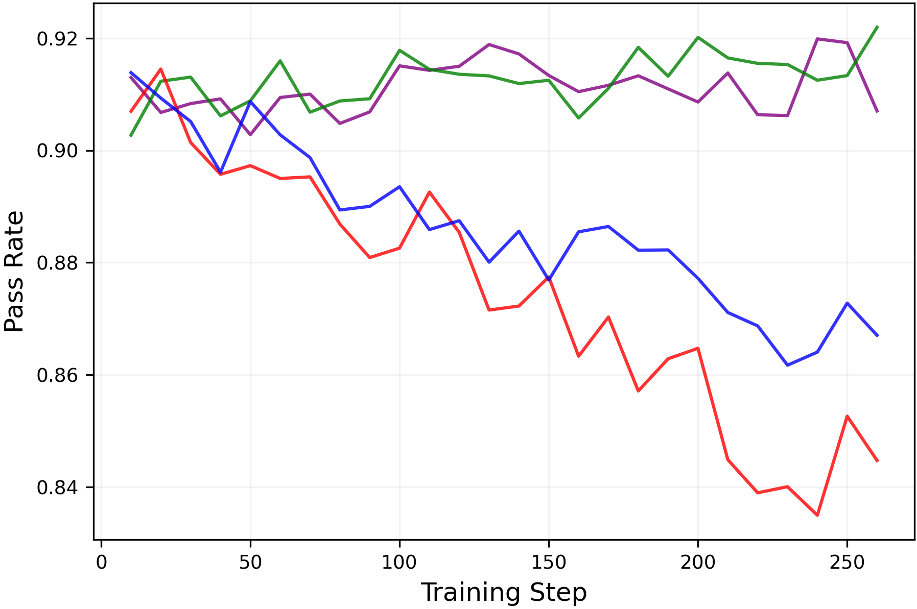
Figure 7:Performance measured by themean@32metric(left)andpass@32metric(right)metric during RLVR for theQwen2.5-7B-Instructmodel trained withDAPO-Math-17kdataset, evaluated on theAMCandMATH-500datasets.

4Conclusion

In this work, we reveal that the clipping mechanism in PPO and GRPO induces biases on entropy, thereby highlighting an overlooked confounding factor in RLVR. Furthermore, we demonstrate that the entropy can be controlled by appropriately setting the clip-low and clip-high values.

Our findings open up several promising avenues for future research. One is to expand the theory by relaxing the assumptions and filling in the theoretical gaps. Another is to empirically investigate how clipping can be utilized to maximize performance. Notably, such performance optimization may correlate with, but is not equivalent to, simply maintaining an appropriate level of entropy.

References

• Agarwal et al. [2025]Shivam Agarwal, Zimin Zhang, Lifan Yuan, Jiawei Han, and Hao Peng.The unreasonable effectiveness of entropy minimization in LLM reasoning.Neural Information Processing Systems, 2025.
• [2]AI-MO.AI-MO validation AMC (American Mathematics Competitions) dataset.Dataset on Hugging Face.URLhttps://huggingface.co/datasets/AI-MO/aimo-validation-amc.
• Burda et al. [2019]Yuri Burda, Harrison Edwards, Amos Storkey, and Oleg Klimov.Exploration by random network distillation.InInternational Conference on Learning Representations, 2019.
• Chen et al. [2021]Mark Chen, Jerry Tworek, Heewoo Jun, Qiming Yuan, Henrique Ponde De Oliveira Pinto, Jared Kaplan, Harri Edwards, Yuri Burda, Nicholas Joseph, Greg Brockman, et al.Evaluating large language models trained on code.arXiv:2107.03374, 2021.
• Chen et al. [2025]Zhipeng Chen, Xiaobo Qin, Youbin Wu, Yue Ling, Qinghao Ye, Wayne Xin Zhao, and Guang Shi.Pass@k training for adaptively balancing exploration and exploitation of large reasoning models.arXiv:2508.10751, 2025.
• Cheng et al. [2025]Daixuan Cheng, Shaohan Huang, Xuekai Zhu, Bo Dai, Wayne Xin Zhao, Zhenliang Zhang, and Furu Wei.Reasoning with exploration: An entropy perspective.arXiv:2506.14758, 2025.
• Cobbe et al. [2021]Karl Cobbe, Vineet Kosaraju, Mohammad Bavarian, Mark Chen, Heewoo Jun, Lukasz Kaiser, Matthias Plappert, Jerry Tworek, Jacob Hilton, Reiichiro Nakano, et al.Training verifiers to solve math word problems.arXiv:2110.14168, 2021.
• Cui et al. [2025]Ganqu Cui, Yuchen Zhang, Jiacheng Chen, Lifan Yuan, Zhi Wang, Yuxin Zuo, Haozhan Li, Yuchen Fan, Huayu Chen, Weize Chen, Zhiyuan Liu, Hao Peng, Lei Bai, Wanli Ouyang, Yu Cheng, Bowen Zhou, and Ning Ding.The entropy mechanism of reinforcement learning for reasoning language models.arXiv:2505.22617, 2025.
• Deng et al. [2025]Jia Deng, Jie Chen, Zhipeng Chen, Wayne Xin Zhao, and Ji-Rong Wen.Decomposing the entropy-performance exchange: The missing keys to unlocking effective reinforcement learning.arXiv:2508.02260, 2025.
• Gao et al. [2025a]Jingtong Gao, Ling Pan, Yejing Wang, Rui Zhong, Chi Lu, Qingpeng Cai, Peng Jiang, and Xiangyu Zhao.Navigate the unknown: Enhancing LLM reasoning with intrinsic motivation guided exploration.arXiv:2505.17621, 2025a.
• Gao et al. [2025b]Zitian Gao, Lynx Chen, Haoming Luo, Joey Zhou, and Bryan Dai.One-shot entropy minimization.arXiv:2505.20282, 2025b.
• Grattafiori et al. [2024]Aaron Grattafiori, Abhimanyu Dubey, Abhinav Jauhri, Abhinav Pandey, Abhishek Kadian, Ahmad Al-Dahle, Aiesha Letman, Akhil Mathur, Alan Schelten, Alex Vaughan, et al.The llama 3 herd of models.arXiv preprint arXiv:2407.21783, 2024.
• Guo et al. [2025]Daya Guo, Dejian Yang, Haowei Zhang, Junxiao Song, Ruoyu Zhang, Runxin Xu, Qihao Zhu, Shirong Ma, Peiyi Wang, and Xiao et al. Bi.DeepSeek-R1 incentivizes reasoning in LLMs through reinforcement learning.Nature, 645:633–638, 2025.
• Haarnoja et al. [2018]Tuomas Haarnoja, Aurick Zhou, Pieter Abbeel, and Sergey Levine.Soft actor-critic: Off-policy maximum entropy deep reinforcement learning with a stochastic actor.International Conference on Machine Learning, 2018.
• He et al. [2025]Andre He, Daniel Fried, and Sean Welleck.Rewarding the unlikely: Lifting grpo beyond distribution sharpening.arXiv:2506.02355, 2025.
• Hendrycks et al. [2021]Dan Hendrycks, Collin Burns, Saurav Kadavath, Akul Arora, Steven Basart, Eric Tang, Dawn Song, and Jacob Steinhardt.Measuring mathematical problem solving with the MATH dataset.Neural Information Processing Systems Track on Datasets and Benchmarks, 2021.
• HuggingFace [2025]HuggingFace.Math-verify.GitHub repository, 2025.URLhttps://github.com/huggingface/Math-Verify.
• HuggingFaceH [4]HuggingFaceH4.Aime 2024 dataset.Dataset on Hugging Face.URLhttps://huggingface.co/datasets/HuggingFaceH4/aime_2024.
• Kakade [2001]Sham M. Kakade.A natural policy gradient.Advances in Neural Information Processing Systems, 2001.
• Lambert et al. [2024]Nathan Lambert, Jacob Morrison, Valentina Pyatkin, Shengyi Huang, Hamish Ivison, Faeze Brahman, Lester James V Miranda, Alisa Liu, Nouha Dziri, Shane Lyu, et al.Tulu 3: Pushing frontiers in open language model post-training.arXiv:2411.15124, 2024.
• Liu [2025]Jiacai Liu.How does RL policy entropy converge during iteration?Zhihu Zhuanlan, 2025.URLhttps://zhuanlan.zhihu.com/p/28476703733.
• Liu et al. [2025a]Mingjie Liu, Shizhe Diao, Ximing Lu, Jian Hu, Xin Dong, Yejin Choi, Jan Kautz, and Yi Dong.ProRL: Prolonged reinforcement learning expands reasoning boundaries in large language models.Neural Information Processing Systems, 2025a.
• Liu et al. [2025b]Zichen Liu, Changyu Chen, Wenjun Li, Penghui Qi, Tianyu Pang, Chao Du, Wee Sun Lee, and Min Lin.Understanding R1-Zero-like training: A critical perspective.Conference on Language Modeling, 2025b.
• Luong et al. [2024]Trung Quoc Luong, Xinbo Zhang, Zhanming Jie, Peng Sun, Xiaoran Jin, and Hang Li.ReFT: Reasoning with reinforced fine-tuning.Association for Computational Linguistics, 2024.
• Lv et al. [2025]Ang Lv, Ruobing Xie, Xingwu Sun, Zhanhui Kang, and Rui Yan.The climb carves wisdom deeper than the summit: On the noisy rewards in learning to reason.arXiv:2505.22653, 2025.
• Schulman et al. [2015]John Schulman, Sergey Levine, Pieter Abbeel, Michael Jordan, and Philipp Moritz.Trust region policy optimization.International Conference on Machine Learning, 2015.
• Schulman et al. [2017]John Schulman, Filip Wolski, Prafulla Dhariwal, Alec Radford, and Oleg Klimov.Proximal policy optimization algorithms.arXiv:1707.06347, 2017.
• Shao et al. [2025]Rulin Shao, Shuyue Stella Li, Rui Xin, Scott Geng, Yiping Wang, Sewoong Oh, Simon Shaolei Du, Nathan Lambert, Sewon Min, Ranjay Krishna, Yulia Tsvetkov, Hannaneh Hajishirzi, Pang Wei Koh, and Luke Zettlemoyer.Spurious rewards: Rethinking training signals in RLVR.arXiv:2506.10947, 2025.
• Shao et al. [2024]Zhihong Shao, Peiyi Wang, Qihao Zhu, Runxin Xu, Junxiao Song, Xiao Bi, Haowei Zhang, Mingchuan Zhang, Y. K. Li, et al.DeepSeekMath: Pushing the limits of mathematical reasoning in open language models.arXiv:2402.03300, 2024.
• Sheng et al. [2025]Guangming Sheng, Chi Zhang, Zilingfeng Ye, Xibin Wu, Wang Zhang, Ru Zhang, Yanghua Peng, Haibin Lin, and Chuan Wu.HybridFlow: A flexible and efficient RLHF framework.European Conference on Computer Systems, 2025.
• Song et al. [2025]Yuda Song, Julia Kempe, and Remi Munos.Outcome-based exploration for LLM reasoning.arXiv:2509.06941, 2025.
• Wang et al. [2025]Yiping Wang, Qing Yang, Zhiyuan Zeng, Liliang Ren, Liyuan Liu, Baolin Peng, Hao Cheng, Xuehai He, Kuan Wang, Jianfeng Gao, Weizhu Chen, Shuohang Wang, Simon Shaolei Du, and Yelong Shen.Reinforcement learning for reasoning in large language models with one training example.Neural Information Processing Systems, 2025.
• Wen et al. [2025]Xumeng Wen, Zihan Liu, Shun Zheng, Zhijian Xu, Shengyu Ye, Zhirong Wu, Xiao Liang, Yang Wang, Junjie Li, Ziming Miao, et al.Reinforcement learning with verifiable rewards implicitly incentivizes correct reasoning in base LLMs.arXiv:2506.14245, 2025.
• Williams [1992]Ronald J. Williams.Simple statistical gradient-following algorithms for connectionist reinforcement learning.Machine Learning, 8(3):229–256, 1992.
• Wu et al. [2025]Fang Wu, Weihao Xuan, Ximing Lu, Zaid Harchaoui, and Yejin Choi.The invisible leash: Why RLVR may not escape its origin.arXiv:2507.14843, 2025.
• Yang et al. [2024]An Yang, Baosong Yang, Beichen Zhang, Binyuan Hui, Bo Zheng, Bowen Yu, Chengyuan Li, Dayiheng Liu, Fei Huang, Guanting Dong, Haoran Wei, Huan Lin, Jian Yang, Jianhong Tu, Jianwei Zhang, Jianxin Yang, Jiaxin Yang, Jingren Zhou, Junyang Lin, Kai Dang, Keming Lu, Keqin Bao, Kexin Yang, Le Yu, Mei Li, Mingfeng Xue, Pei Zhang, Qin Zhu, Rui Men, Runji Lin, Tianhao Li, Tingyu Xia, Xingzhang Ren, Xuancheng Ren, Yang Fan, Yang Su, Yi-Chao Zhang, Yunyang Wan, Yuqi Liu, Zeyu Cui, Zhenru Zhang, Zihan Qiu, Shanghaoran Quan, and Zekun Wang.Qwen2.5 technical report.arXiv:2412.15115, 2024.
• Yang et al. [2025]An Yang, Anfeng Li, Baosong Yang, Beichen Zhang, Binyuan Hui, Bo Zheng, Bowen Yu, Chang Gao, Chengen Huang, Chenxu Lv, et al.Qwen3 technical report.arXiv:2505.09388, 2025.
• Yu et al. [2025]Qiying Yu, Zheng Zhang, Ruofei Zhu, Yufeng Yuan, Xiaochen Zuo, Yu Yue, Weinan Dai, Tiantian Fan, Gaohong Liu, Lingjun Liu, Xin Liu, Haibin Lin, Zhiqi Lin, Bole Ma, Guangming Sheng, Yuxuan Tong, Chi Zhang, Mofan Zhang, Wang Zhang, Hang Zhu, Jinhua Zhu, Jiaze Chen, Jiangjie Chen, Chengyi Wang, Hongli Yu, Yuxuan Song, Xiangpeng Wei, Hao Zhou, Jingjing Liu, Wei-Ying Ma, Ya-Qin Zhang, Lin Yan, Mu Qiao, Yonghui Wu, and Mingxuan Wang.DAPO: An open-source LLM reinforcement learning system at scale.Neural Information Processing Systems, 2025.
• Yue et al. [2025]Yang Yue, Zhiqi Chen, Rui Lu, Andrew Zhao, Zhaokai Wang, Shiji Song, and Gao Huang.Does reinforcement learning really incentivize reasoning capacity in LLMs beyond the base model?Neural Information Processing Systems, 2025.
• Zhao et al. [2025]Xuandong Zhao, Zhewei Kang, Aosong Feng, Sergey Levine, and Dawn Song.Learning to reason without external rewards.arXiv:2505.19590, 2025.
• Zhu et al. [2025]Xinyu Zhu, Mengzhou Xia, Zhepei Wei, Wei-Lin Chen, Danqi Chen, and Yu Meng.The surprising effectiveness of negative reinforcement in LLM reasoning.Neural Information Processing Systems, 2025.

Appendix AAnalysis of policy gradient: Proof of Theorem1

Here we present the proof for Theorem1.

Proof.

We first analyze the first-order Taylor expansion of entropy relative to logit change (Δθs,a=θs,ak+1−θs,ak)\Delta\theta_{s,a}=\theta^{k+1}_{s,a}-\theta^{k}_{s,a}). This first step is closely inspired byLiu [2025]. We can Taylor expand the entropy with respect toΔ​θ\Delta\theta:

ℋ​(θk+1|s)=ℋ​(θk|s)+⟨∇θℋ​(θk|s),Δ​θ⟩+𝒪​((Δ​θ)2)\mathcal{H}(\theta^{k+1}|s)=\mathcal{H}(\theta^{k}|s)+\left\langle\nabla_{\theta}\mathcal{H}(\theta^{k}|s),\ \Delta\theta\right\rangle+\mathcal{O}((\Delta\theta)^{2})The gradient of policy entropy is

∇θℋ​(θ|s)\displaystyle\nabla_{\theta}\mathcal{H}(\theta|s)=∇θ(−𝔼a∼πθ(⋅|s)​[log⁡πθ​(a|s)])\displaystyle=\nabla_{\theta}\left(-\mathbb{E}_{a\sim\pi_{\theta}(\cdot|s)}[\log\pi_{\theta}(a|s)]\right)=−𝔼a∼πθ(⋅|s)​[∇θlog⁡πθ​(a|s)+log⁡πθ​(a|s)​∇θlog⁡πθ​(a|s)]\displaystyle=-\mathbb{E}_{a\sim\pi_{\theta}(\cdot|s)}\left[\nabla_{\theta}\log\pi_{\theta}(a|s)+\log\pi_{\theta}(a|s)\nabla_{\theta}\log\pi_{\theta}(a|s)\right]=−𝔼a∼πθ(⋅|s)​[log⁡πθ​(a|s)​∇θlog⁡πθ​(a|s)].\displaystyle=-\mathbb{E}_{a\sim\pi_{\theta}(\cdot|s)}\left[\log\pi_{\theta}(a|s)\nabla_{\theta}\log\pi_{\theta}(a|s)\right]. Therefore, we have

⟨∇θℋ​(θk|s),θk+1−θk⟩\displaystyle\left\langle\nabla_{\theta}\mathcal{H}(\theta^{k}|s),\theta^{k+1}-\theta^{k}\right\rangle=−⟨𝔼a∼πk(⋅|s)​[log⁡πk​(a|s)​∇θlog⁡πk​(a|s)],θk+1−θk⟩\displaystyle=-\left\langle\mathbb{E}_{a\sim\pi_{k}(\cdot|s)}\left[\log\pi_{k}(a|s)\nabla_{\theta}\log\pi_{k}(a|s)\right],\ \theta^{k+1}-\theta^{k}\right\rangle=−𝔼a∼πk(⋅|s)​[log⁡πk​(a|s)​⟨∇θlog⁡πk​(a|s),θk+1−θk⟩]\displaystyle=-\mathbb{E}_{a\sim\pi_{k}(\cdot|s)}\left[\log\pi_{k}(a|s)\left\langle\nabla_{\theta}\log\pi_{k}(a|s),\ \theta^{k+1}-\theta^{k}\right\rangle\right]=−𝔼a∼πk(⋅|s)​[log⁡πk​(a|s)​∑s′∈𝒮,a′∈𝒜∂log⁡πk​(a|s)∂θs′,a′⋅(θs′,a′k+1−θs′,a′k)]\displaystyle=-\mathbb{E}_{a\sim\pi_{k}(\cdot|s)}\left[\log\pi_{k}(a|s)\sum_{s^{\prime}\in\mathcal{S},a^{\prime}\in\mathcal{A}}\frac{\partial\log\pi_{k}(a|s)}{\partial\theta_{s^{\prime},a^{\prime}}}\cdot\left(\theta^{k+1}_{s^{\prime},a^{\prime}}-\theta^{k}_{s^{\prime},a^{\prime}}\right)\right]=−∑s′∈𝒮,a′∈𝒜𝔼a∼πk(⋅|s)​[log⁡πk​(a|s)⋅∂log⁡πk​(a|s)∂θs′,a′]⋅(θs′,a′k+1−θs′,a′k)\displaystyle=-\sum_{s^{\prime}\in\mathcal{S},a^{\prime}\in\mathcal{A}}\mathbb{E}_{a\sim\pi_{k}(\cdot|s)}\left[\log\pi_{k}(a|s)\cdot\frac{\partial\log\pi_{k}(a|s)}{\partial\theta_{s^{\prime},a^{\prime}}}\right]\cdot\left(\theta^{k+1}_{s^{\prime},a^{\prime}}-\theta^{k}_{s^{\prime},a^{\prime}}\right)=−∑s′∈𝒮,a′∈𝒜(θs′,a′k+1−θs′,a′k)⋅𝔼a∼πk(⋅|s)​[log⁡πk​(a|s)⋅∂log⁡πθ​(a|s)∂θs′,a′]\displaystyle=-\sum_{s^{\prime}\in\mathcal{S},a^{\prime}\in\mathcal{A}}\left(\theta^{k+1}_{s^{\prime},a^{\prime}}-\theta^{k}_{s^{\prime},a^{\prime}}\right)\cdot\mathbb{E}_{a\sim\pi_{k}(\cdot|s)}\left[\log\pi_{k}(a|s)\cdot\frac{\partial\log\pi_{\theta}(a|s)}{\partial\theta_{s^{\prime},a^{\prime}}}\right]=(⋆)−∑s′∈𝒮,a′∈𝒜(θs′,a′k+1−θs′,a′k)⋅𝟏{s=s′}⋅πk​(a′|s)​(log⁡πk​(a′|s)−𝔼a∼πk(⋅|s)​[log⁡πk​(a|s)])\displaystyle\overset{(\star)}{=}-\sum_{s^{\prime}\in\mathcal{S},a^{\prime}\in\mathcal{A}}\left(\theta^{k+1}_{s^{\prime},a^{\prime}}-\theta^{k}_{s^{\prime},a^{\prime}}\right)\cdot\mathbf{1}_{\{s=s^{\prime}\}}\cdot\pi_{k}(a^{\prime}|s)\left(\log\pi_{k}(a^{\prime}|s)-\mathbb{E}_{a\sim\pi_{k}(\cdot|s)}[\log\pi_{k}(a|s)]\right)where the final equation holds from the derivation below.

𝔼a∼πk(⋅|s)​[log⁡πk​(a|s)⋅∂log⁡πθ​(a|s)∂θs′,a′]\displaystyle\mathbb{E}_{a\sim\pi_{k}(\cdot|s)}\left[\log\pi_{k}(a|s)\cdot\frac{\partial\log\pi_{\theta}(a|s)}{\partial\theta_{s^{\prime},a^{\prime}}}\right]=𝔼a∼πk(⋅|s)​[log⁡πk​(a|s)⋅∂∂θs′,a′​(θs,a−log⁡(∑a∈𝒜exp⁡{θs,a}))]\displaystyle=\mathbb{E}_{a\sim\pi_{k}(\cdot|s)}\left[\log\pi_{k}(a|s)\cdot\frac{\partial}{\partial\theta_{s^{\prime},a^{\prime}}}\left(\theta_{s,a}-\log\left(\sum_{a\in\mathcal{A}}\exp\{\theta_{s,a}\}\right)\right)\right]=𝔼a∼πk(⋅|s)​[log⁡πk​(a|s)⋅𝟏{s=s′}⋅(𝟏{a=a′}−πk​(a′|s))]\displaystyle=\mathbb{E}_{a\sim\pi_{k}(\cdot|s)}\left[\log\pi_{k}(a|s)\cdot\mathbf{1}_{\{s=s^{\prime}\}}\cdot\left(\mathbf{1}_{\{a=a^{\prime}\}}-\pi_{k}(a^{\prime}|s)\right)\right]=𝟏{s=s′}⋅𝔼a∼πk(⋅|s)​[log⁡πk​(a|s)⋅(𝟏{a=a′}−πk​(a′|s))]\displaystyle=\mathbf{1}_{\{s=s^{\prime}\}}\cdot\mathbb{E}_{a\sim\pi_{k}(\cdot|s)}\left[\log\pi_{k}(a|s)\cdot\left(\mathbf{1}_{\{a=a^{\prime}\}}-\pi_{k}(a^{\prime}|s)\right)\right]=𝟏{s=s′}⋅[πk​(a′|s)​log⁡πk​(a′|s)−πk​(a′|s)⋅𝔼a∼πk(⋅|s)​[log⁡πk​(a|s)]].\displaystyle=\mathbf{1}_{\{s=s^{\prime}\}}\cdot\left[\pi_{k}(a^{\prime}|s)\log\pi_{k}(a^{\prime}|s)-\pi_{k}(a^{\prime}|s)\cdot\mathbb{E}_{a\sim\pi_{k}(\cdot|s)}\left[\log\pi_{k}(a|s)\right]\right].Hence, we obtain the first-order Taylor expansion of policy entropy:

ℋ​(θk+1|s)−ℋ​(θk|s)=−𝔼a∼πk(⋅|s)​[(θs,ak+1−θs,ak)​(log⁡πk​(a|s)+ℋ​(θk|s))]+𝒪​((Δ​θ)2).\mathcal{H}(\theta^{k+1}|s)-\mathcal{H}(\theta^{k}|s)=-\mathbb{E}_{a\sim\pi_{k}(\cdot|s)}\left[\left(\theta^{k+1}_{s,a}-\theta^{k}_{s,a}\right)\left(\log\pi_{k}(a|s)+\mathcal{H}(\theta^{k}|s)\right)\right]+\mathcal{O}((\Delta\theta)^{2}).(9) For our next step (and this is where the technical novelty of our analysis begins), we express the logit changeΔ​θ\Delta\thetain terms of clipping events. Consider the clipped surrogate objective

𝒥​(θ)=𝔼x∼𝒟,τ∼πo​l​d(⋅|x),A​[1T​∑t=0TCε​(rt,At)]\mathcal{J}(\theta)=\mathbb{E}_{x\sim\mathcal{D},\tau\sim\pi_{old}(\cdot|x),A}\left[\frac{1}{T}\sum_{t=0}^{T}C_{\varepsilon}(r_{t},A_{t})\right]wherert=πθ​(yt|y<t,x)πo​l​d​(yt|y<t,x)r_{t}=\frac{\pi_{\theta}(y_{t}|y_{<t},x)}{\pi_{old}(y_{t}|y_{<t},x)}. Now we compute the partial derivative of𝒥​(θ)\mathcal{J}(\theta)over eachθs,a\theta_{s,a}. Here sinceπθ​(a|s)\pi_{\theta}(a|s)is a function ofθ⋅,s\theta_{\cdot,s},Cε​(rt,At)C_{\varepsilon}(r_{t},A_{t})is a constant with respect toθs,a\theta_{s,a}unlesss=(y<t,x)s=(y_{<t},x). Therefore

∂∂θs,a​𝒥​(θ)\displaystyle\frac{\partial}{\partial\theta_{s,a}}\mathcal{J}(\theta)=𝔼x∼𝒟,τ∼πo​l​d(⋅|x),A​[1T​∂∂θs,a​∑t=0TCε​(rt,At)]\displaystyle=\mathbb{E}_{x\sim\mathcal{D},\tau\sim\pi_{old}(\cdot|x),A}\left[\frac{1}{T}\frac{\partial}{\partial\theta_{s,a}}\sum_{t=0}^{T}C_{\varepsilon}(r_{t},A_{t})\right]=𝔼x∼𝒟,τ∼πo​l​d(⋅|x),A​[1T​∑t=0T∂∂θs,a​𝟏{(y<t,x)=s}​Cε​(rt,At)]\displaystyle=\mathbb{E}_{x\sim\mathcal{D},\tau\sim\pi_{old}(\cdot|x),A}\left[\frac{1}{T}\sum_{t=0}^{T}\frac{\partial}{\partial\theta_{s,a}}\mathbf{1}_{\{(y_{<t},x)=s\}}C_{\varepsilon}(r_{t},A_{t})\right]=𝔼x∼𝒟,yt∼πo​l​d(⋅|y<t,x),At​[𝟏{(y<t,x)=s}​∂∂θs,a​Cε​(rt,At)]\displaystyle=\mathbb{E}_{x\sim\mathcal{D},y_{t}\sim\pi_{old}(\cdot|y_{<t},x),A_{t}}\left[\mathbf{1}_{\{(y_{<t},x)=s\}}\frac{\partial}{\partial\theta_{s,a}}C_{\varepsilon}(r_{t},A_{t})\right]=dπo​l​d​(s)×𝔼a′∼πo​l​d(⋅|s),A​[∂∂θs,a​Cε​(r​(s,a′),A)]\displaystyle=d^{\pi_{old}}(s)\times\mathbb{E}_{a^{\prime}\sim\pi_{old}(\cdot|s),A}\left[\frac{\partial}{\partial\theta_{s,a}}C_{\varepsilon}(r(s,a^{\prime}),A)\right]wheredπo​l​d​(s)d^{\pi_{old}}(s)is the state-visiting probability under the policyπo​l​d\pi_{old}. Thus we can write

1dπo​l​d​(s)​∂∂θs,ak​𝒥​(θ)=𝔼x∼𝒟,a′∼πo​l​d(⋅|s),A​[∂∂θs,a​Cε​(r​(s,a′),A)]\displaystyle\frac{1}{d^{\pi_{old}}(s)}\frac{\partial}{\partial\theta_{s,a}^{k}}\mathcal{J}(\theta)=\mathbb{E}_{x\sim\mathcal{D},a^{\prime}\sim\pi_{old}(\cdot|s),A}\left[\frac{\partial}{\partial\theta_{s,a}}C_{\varepsilon}(r(s,a^{\prime}),A)\right]=ℙ​(A>0)​𝔼a′∼πo​l​d(⋅|s),A​[∂∂θs,a​Cε​(r​(s,a′),A)​∣A>​0]+ℙ​(A<0)​𝔼a′∼πo​l​d(⋅|s),A​[∂∂θs,a​Cε​(r​(s,a′),A)∣A<0]\displaystyle=\mathbb{P}(A>0)\mathbb{E}_{a^{\prime}\sim\pi_{old}(\cdot|s),A}\left[\frac{\partial}{\partial\theta_{s,a}}C_{\varepsilon}(r(s,a^{\prime}),A)\mid A>0\right]+\mathbb{P}(A<0)\mathbb{E}_{a^{\prime}\sim\pi_{old}(\cdot|s),A}\left[\frac{\partial}{\partial\theta_{s,a}}C_{\varepsilon}(r(s,a^{\prime}),A)\mid A<0\right]=ℙ​(A>0,1−ε<r​(s,a′)<1+ε)​𝔼a′∼πo​l​d(⋅|s),A​[∂∂θs,a​Cε​(r​(s,a′),A)​∣A>​0,1−ε<r​(s,a′)<1+ε]\displaystyle=\mathbb{P}(A>0,1-\varepsilon<r(s,a^{\prime})<1+\varepsilon)\mathbb{E}_{a^{\prime}\sim\pi_{old}(\cdot|s),A}\left[\frac{\partial}{\partial\theta_{s,a}}C_{\varepsilon}(r(s,a^{\prime}),A)\mid A>0,1-\varepsilon<r(s,a^{\prime})<1+\varepsilon\right]+ℙ​(A>0,1+ε<r​(s,a′))​𝔼a′∼πo​l​d(⋅|s),A​[∂∂θs,a​Cε​(r​(s,a′),A)​∣A>​0,1+ε<r​(s,a′)]\displaystyle\quad+\mathbb{P}(A>0,1+\varepsilon<r(s,a^{\prime}))\mathbb{E}_{a^{\prime}\sim\pi_{old}(\cdot|s),A}\left[\frac{\partial}{\partial\theta_{s,a}}C_{\varepsilon}(r(s,a^{\prime}),A)\mid A>0,1+\varepsilon<r(s,a^{\prime})\right]+ℙ​(A>0,0≤r​(s,a′)<1−ε)​𝔼a′∼πo​l​d(⋅|s),A​[∂∂θs,a​Cε​(r​(s,a′),A)​∣A>​0,0≤r​(s,a′)<1−ε]\displaystyle+\mathbb{P}(A>0,0\leq r(s,a^{\prime})<1-\varepsilon)\mathbb{E}_{a^{\prime}\sim\pi_{old}(\cdot|s),A}\left[\frac{\partial}{\partial\theta_{s,a}}C_{\varepsilon}(r(s,a^{\prime}),A)\mid A>0,0\leq r(s,a^{\prime})<1-\varepsilon\right]+ℙ​(A<0,1−ε<r​(s,a′)<1+ε)​𝔼a′∼πo​l​d(⋅|s),A​[∂∂θs,a​Cε​(r​(s,a′),A)∣A<0,0≤r​(s,a′)<1−ε]\displaystyle+\mathbb{P}(A<0,1-\varepsilon<r(s,a^{\prime})<1+\varepsilon)\mathbb{E}_{a^{\prime}\sim\pi_{old}(\cdot|s),A}\left[\frac{\partial}{\partial\theta_{s,a}}C_{\varepsilon}(r(s,a^{\prime}),A)\mid A<0,0\leq r(s,a^{\prime})<1-\varepsilon\right]+ℙ​(A<0,1+ε<r​(s,a′))​𝔼a′∼πo​l​d(⋅|s),A​[∂∂θs,a​Cε​(r​(s,a′),A)∣A<0,1+ε<r​(s,a′)]\displaystyle+\mathbb{P}(A<0,1+\varepsilon<r(s,a^{\prime}))\mathbb{E}_{a^{\prime}\sim\pi_{old}(\cdot|s),A}\left[\frac{\partial}{\partial\theta_{s,a}}C_{\varepsilon}(r(s,a^{\prime}),A)\mid A<0,1+\varepsilon<r(s,a^{\prime})\right]+ℙ​(A<0,0≤r​(s,a)<1−ε)​𝔼a′∼πo​l​d(⋅|s),A​[∂∂θs,a​Cε​(r​(s,a′),A)∣A<0,0≤r​(s,a′)<1−ε]\displaystyle+\mathbb{P}(A<0,0\leq r(s,a)<1-\varepsilon)\mathbb{E}_{a^{\prime}\sim\pi_{old}(\cdot|s),A}\left[\frac{\partial}{\partial\theta_{s,a}}C_{\varepsilon}(r(s,a^{\prime}),A)\mid A<0,0\leq r(s,a^{\prime})<1-\varepsilon\right]+ℙ​(A=0)​𝔼a′∼πo​l​d(⋅|s),A​[∂∂θs,a​Cε​(r​(s,a′),A)∣A=0]\displaystyle+\mathbb{P}(A=0)\mathbb{E}_{a^{\prime}\sim\pi_{old}(\cdot|s),A}\left[\frac{\partial}{\partial\theta_{s,a}}C_{\varepsilon}(r(s,a^{\prime}),A)\mid A=0\right]=ℙ​(A>0,1−ε<r​(s,a′)<1+ε)​𝔼a′∼πo​l​d(⋅|s),A​[∂∂θs,a​r​(s,a′)⋅A​∣A>​0,1−ε<r​(s,a′)<1+ε]\displaystyle=\mathbb{P}(A>0,1-\varepsilon<r(s,a^{\prime})<1+\varepsilon)\mathbb{E}_{a^{\prime}\sim\pi_{old}(\cdot|s),A}\left[\frac{\partial}{\partial\theta_{s,a}}r(s,a^{\prime})\cdot A\mid A>0,1-\varepsilon<r(s,a^{\prime})<1+\varepsilon\right]+ℙ​(A>0,1+ε<r​(s,a′))​𝔼a∼πo​l​d(⋅|s),A​[∂∂θs,a​(1+ε)⋅A​∣A>​0,1+ε<r​(s,a′)]\displaystyle+\mathbb{P}(A>0,1+\varepsilon<r(s,a^{\prime}))\mathbb{E}_{a\sim\pi_{old}(\cdot|s),A}\left[\frac{\partial}{\partial\theta_{s,a}}(1+\varepsilon)\cdot A\mid A>0,1+\varepsilon<r(s,a^{\prime})\right]+ℙ​(A>0,0≤r​(s,a′)<1−ε)​𝔼a′∼πo​l​d(⋅|s),A​[∂∂θs,a​r​(s,a′)⋅A​∣A>​0,0<r​(s,a′)<1−ε]\displaystyle+\mathbb{P}(A>0,0\leq r(s,a^{\prime})<1-\varepsilon)\mathbb{E}_{a^{\prime}\sim\pi_{old}(\cdot|s),A}\left[\frac{\partial}{\partial\theta_{s,a}}r(s,a^{\prime})\cdot A\mid A>0,0<r(s,a^{\prime})<1-\varepsilon\right]+ℙ​(A<0,1−ε≤r​(s,a′)<1+ε)​𝔼a′∼πo​l​d(⋅|s),A​[∂∂θs,a​r​(s,a′)⋅A∣A<0,1−ε≤r​(s,a′)<1+ε]\displaystyle+\mathbb{P}(A<0,1-\varepsilon\leq r(s,a^{\prime})<1+\varepsilon)\mathbb{E}_{a^{\prime}\sim\pi_{old}(\cdot|s),A}\left[\frac{\partial}{\partial\theta_{s,a}}r(s,a^{\prime})\cdot A\mid A<0,1-\varepsilon\leq r(s,a^{\prime})<1+\varepsilon\right]+ℙ​(A<0,1+ε<r​(s,a′))​𝔼a′∼πo​l​d(⋅|s),A​[∂∂θs,a​r​(s,a′)⋅A∣A<0,1+ε<r​(s,a′)]\displaystyle+\mathbb{P}(A<0,1+\varepsilon<r(s,a^{\prime}))\mathbb{E}_{a^{\prime}\sim\pi_{old}(\cdot|s),A}\left[\frac{\partial}{\partial\theta_{s,a}}r(s,a^{\prime})\cdot A\mid A<0,1+\varepsilon<r(s,a^{\prime})\right]+ℙ​(A<0,0≤r​(s,a′)<1−ε)​𝔼a′∼πo​l​d(⋅|s),A​[∂∂θs,a​(1−ε)⋅A∣A<0,0≤r​(s,a′)<1−ε]\displaystyle+\mathbb{P}(A<0,0\leq r(s,a^{\prime})<1-\varepsilon)\mathbb{E}_{a^{\prime}\sim\pi_{old}(\cdot|s),A}\left[\frac{\partial}{\partial\theta_{s,a}}(1-\varepsilon)\cdot A\mid A<0,0\leq r(s,a^{\prime})<1-\varepsilon\right] Note thatAAis independent ofπo​l​d\pi_{old}, and that𝔼​[A]=0\mathbb{E}[A]=0. Denote𝔼​[A​|A>​0]=μ=−𝔼​[A|A<0]\mathbb{E}[A|A>0]=\mu=-\mathbb{E}[A|A<0]andℙ​(A>0)=ℙ​(A<0)=ν\mathbb{P}(A>0)=\mathbb{P}(A<0)=\nu. Then the symmetric terms cross out, resulting in

∂∂θs,a​𝒥​(θ)\displaystyle\frac{\partial}{\partial\theta_{s,a}}\mathcal{J}(\theta)=ℙ​(A>0,0≤r​(s,a)<1−ε)​𝔼a∼πo​l​d(⋅|s),A​[∂∂θs,a​r​(s,a)⋅A​∣A>​0,0≤r​(s,a)<1−ε]\displaystyle=\mathbb{P}(A>0,0\leq r(s,a)<1-\varepsilon)\mathbb{E}_{a\sim\pi_{old}(\cdot|s),A}\left[\frac{\partial}{\partial\theta_{s,a}}r(s,a)\cdot A\mid A>0,0\leq r(s,a)<1-\varepsilon\right]+ℙ​(A<0,1+ε<r​(s,a))​𝔼a∼πo​l​d(⋅|s),A​[∂∂θs,a​r​(s,a)⋅A∣A<0,1+ε<r​(s,a)]\displaystyle+\mathbb{P}(A<0,1+\varepsilon<r(s,a))\mathbb{E}_{a\sim\pi_{old}(\cdot|s),A}\left[\frac{\partial}{\partial\theta_{s,a}}r(s,a)\cdot A\mid A<0,1+\varepsilon<r(s,a)\right]=μ​ν​ℙ​(0≤r​(s,a)<1−ε)​𝔼a∼πo​l​d(⋅|s)​[∂∂θs,a​r​(s,a)∣0≤r​(s,a)<1−ε]\displaystyle=\mu\nu\mathbb{P}(0\leq r(s,a)<1-\varepsilon)\mathbb{E}_{a\sim\pi_{old}(\cdot|s)}\left[\frac{\partial}{\partial\theta_{s,a}}r(s,a)\mid 0\leq r(s,a)<1-\varepsilon\right]−μ​ν​ℙ​(1+ε<r​(s,a))​𝔼a∼πo​l​d(⋅|s)​[∂∂θs,a​r​(s,a)∣1+ε<r​(s,a)]\displaystyle-\mu\nu\mathbb{P}(1+\varepsilon<r(s,a))\mathbb{E}_{a\sim\pi_{old}(\cdot|s)}\left[\frac{\partial}{\partial\theta_{s,a}}r(s,a)\mid 1+\varepsilon<r(s,a)\right] Recall that withrk​(s,a)=πk​(a|s)πo​l​d​(a|s)r_{k}(s,a)=\frac{\pi_{k}(a|s)}{\pi_{old}(a|s)}, the probabilistic events corresponding to clipping are denoted as:

Xk​(s)\displaystyle X_{k}(s)={a∈𝒜​(s)|rk​(s,a)<1−εlow}\displaystyle=\{a\in\mathcal{A}(s)\ |\ r_{k}(s,a)<1-\varepsilon_{\mathrm{low}}\}Yk​(s)\displaystyle Y_{k}(s)={a∈𝒜​(s)|rk​(s,a)>1+εhigh}.\displaystyle=\{a\in\mathcal{A}(s)\ |\ r_{k}(s,a)>1+\varepsilon_{\mathrm{high}}\}. Then the above expression simplifies into

∂∂θs,a​𝒥​(θk)\displaystyle\frac{\partial}{\partial\theta_{s,a}}\mathcal{J}(\theta^{k})=μ​ν​dπo​l​d​(s)​𝔼a′∼πo​l​d(⋅|s)​[∂∂θs,a​(πk​(a′|s)πo​l​d​(a′|s))​(𝟏Xk​(s)​(a′)−𝟏Yk​(s)​(a′))]\displaystyle=\mu\nu d^{\pi_{old}}(s)\mathbb{E}_{a^{\prime}\sim\pi_{old}(\cdot|s)}\left[\frac{\partial}{\partial\theta_{s,a}}\Big(\frac{\pi_{k}(a^{\prime}|s)}{\pi_{old}(a^{\prime}|s)}\Big)(\mathbf{1}_{X_{k}(s)}(a^{\prime})-\mathbf{1}_{Y_{k}(s)}(a^{\prime}))\right]where𝟏C​(x)\mathbf{1}_{C}(x)is the indicator function of setCC. Note that the derivative ofπ​(a|s)=exp⁡(θs,a)/∑a′∈𝒜exp⁡(θs,a′)=exp⁡(θs,a)/Z\pi(a|s)=\exp(\theta_{s,a})/\sum_{a^{\prime}\in\mathcal{A}}\exp(\theta_{s,a^{\prime}})=\exp(\theta_{s,a})/Zw.r.t.θ\thetais

∂πθ​(a′|s′)θs,a\displaystyle\frac{\partial\pi_{\theta}(a^{\prime}|s^{\prime})}{\theta_{s,a}}={𝟏{s=s′}⋅(exp⁡(θs,a)Z−exp⁡(2​θs,a)Z2)if​a′=a−𝟏{s=s′}⋅(exp⁡(θs,a+θ​s,a′)Z2)if​a′≠a\displaystyle=\begin{cases}\mathbf{1}_{\{s=s^{\prime}\}}\cdot\Big(\frac{\exp(\theta_{s,a})}{Z}-\frac{\exp(2\theta_{s,a})}{Z^{2}}\Big)\;&\text{if}\;a^{\prime}=a\\ -\mathbf{1}_{\{s=s^{\prime}\}}\cdot\Big(\frac{\exp(\theta_{s,a}+\theta{s,a^{\prime}})}{Z^{2}}\Big)\;&\text{if}\;a^{\prime}\neq a\end{cases}=𝟏{s=s′}⋅(𝟏{a′=a}​exp⁡(θs,a)Z−exp⁡(θs,a+θs,a′)Z2)\displaystyle=\mathbf{1}_{\{s=s^{\prime}\}}\cdot\Big(\mathbf{1}_{\{a^{\prime}=a\}}\frac{\exp(\theta_{s,a})}{Z}-\frac{\exp(\theta_{s,a}+\theta_{s,a^{\prime}})}{Z^{2}}\Big)=𝟏{s=s′}⋅(𝟏{a′=a}​πθ​(a|s)−πθ​(a|s)⋅πθ​(a′|s))\displaystyle=\mathbf{1}_{\{s=s^{\prime}\}}\cdot\Big(\mathbf{1}_{\{a^{\prime}=a\}}\pi_{\theta}(a|s)-\pi_{\theta}(a|s)\cdot\pi_{\theta}(a^{\prime}|s)\Big)=𝟏{s=s′}​πθ​(a|s)​(𝟏{a′=a}−πθ​(a′|s))\displaystyle=\mathbf{1}_{\{s=s^{\prime}\}}\;\pi_{\theta}(a|s)\Big(\mathbf{1}_{\{a^{\prime}=a\}}-\pi_{\theta}(a^{\prime}|s)\Big)Hence,

∂∂θs,a​𝒥​(θk)\displaystyle\frac{\partial}{\partial\theta_{s,a}}\mathcal{J}(\theta^{k})=μ​ν​dπo​l​d​(s)​𝔼a′∼πo​l​d(⋅|s)​[(𝟏{a=a′}​πk​(a|s)πo​l​d​(a′|s)−πk​(a|s)​πk​(a′|s)πo​l​d​(a′|s))​(𝟏Xk​(s)​(a′)−𝟏Yk​(s)​(a′))]\displaystyle=\mu\nu d^{\pi_{old}}(s)\mathbb{E}_{a^{\prime}\sim\pi_{old}(\cdot|s)}\left[\left(\mathbf{1}_{\{a=a^{\prime}\}}\frac{\pi_{k}(a|s)}{\pi_{old}(a^{\prime}|s)}-\pi_{k}(a|s)\frac{\pi_{k}(a^{\prime}|s)}{\pi_{old}(a^{\prime}|s)}\right)(\mathbf{1}_{X_{k}(s)}(a^{\prime})-\mathbf{1}_{Y_{k}(s)}(a^{\prime}))\right]=μ​ν​dπo​l​d​(s)​∑a′∈𝒜​(s)[(𝟏{a=a′}​πk​(a|s)−πk​(a′|s))​(𝟏Xk​(s)​(a′)−𝟏Yk​(s)​(a′))]\displaystyle=\mu\nu d^{\pi_{old}}(s)\sum_{a^{\prime}\in\mathcal{A}(s)}\left[\left(\mathbf{1}_{\{a=a^{\prime}\}}\pi_{k}(a|s)-\pi_{k}(a^{\prime}|s)\right)(\mathbf{1}_{X_{k}(s)}(a^{\prime})-\mathbf{1}_{Y_{k}(s)}(a^{\prime}))\right]=μ​ν​dπo​l​d​(s)​[πk​(a|s)​(𝟏Xk​(a|s)−𝟏Yk​(s)​(a))−πk​(a|s)​𝔼a′∼πk(⋅|s)​(𝟏Xk​(s)​(a′)−𝟏Yk​(s)​(a′))]\displaystyle=\mu\nu d^{\pi_{old}}(s)\left[\pi_{k}(a|s)(\mathbf{1}_{X_{k}}(a|s)-\mathbf{1}_{Y_{k}(s)}(a))-\pi_{k}(a|s)\mathbb{E}_{a^{\prime}\sim\pi_{k}(\cdot|s)}(\mathbf{1}_{X_{k}(s)}(a^{\prime})-\mathbf{1}_{Y_{k}(s)}(a^{\prime}))\right]=μ​ν​dπo​l​d​(s)⋅πk​(a|s)​[hk​(a|s)−𝔼a′∼πk(⋅|s)​hk​(a′|s)]\displaystyle=\mu\nu d^{\pi_{old}}(s)\cdot\pi_{k}(a|s)\left[h_{k}(a|s)-\mathbb{E}_{a^{\prime}\sim\pi_{k}(\cdot|s)}h_{k}(a^{\prime}|s)\right]where we definehk​(a|s)=𝟏Xk​(s)​(a)−𝟏Yk​(s)​(a)h_{k}(a|s)=\mathbf{1}_{X_{k}(s)}(a)-\mathbf{1}_{Y_{k}(s)}(a).

Recall that as we are assuming gradient descent updates, we update the logits via the policy gradient with respect to the clipped objective

θs,ak+1−θs,ak=η⋅∂∂θs,a​𝒥​(θk),\theta^{k+1}_{s,a}-\theta^{k}_{s,a}=\eta\cdot\frac{\partial}{\partial\theta_{s,a}}\mathcal{J}(\theta^{k}),obtaining the following logit change formula.

θs,ak+1−θs,ak=μ​ν​η​dπo​l​d​(s)​πk​(a|s)​(hk​(a|s)−𝔼a′∼πk(⋅|s)​hk​(a′|s))\theta^{k+1}_{s,a}-\theta^{k}_{s,a}=\mu\nu\eta\;d^{\pi_{old}(s)}\;\pi_{k}(a|s)\left(h_{k}(a|s)-\mathbb{E}_{a^{\prime}\sim\pi_{k}(\cdot|s)}h_{k}(a^{\prime}|s)\right)Now we can plug this this back into (9). By direct calculation, we conclude our proof.

ℋ​(θk+1|s)−ℋ​(θk|s)\displaystyle\mathcal{H}(\theta^{k+1}|s)-\mathcal{H}(\theta^{k}|s)=−𝔼a∼πk(⋅|s)​[(θs,ak+1−θs,ak)​(log⁡πk​(a|s)+ℋ​(θk|s))]+𝒪​((Δ​θ)2)\displaystyle=-\mathbb{E}_{a\sim\pi_{k}(\cdot|s)}\left[\left(\theta^{k+1}_{s,a}-\theta^{k}_{s,a}\right)\left(\log\pi_{k}(a|s)+\mathcal{H}(\theta^{k}|s)\right)\right]+\mathcal{O}((\Delta\theta)^{2})=−μνηdπo​l​d(s)𝔼a∼πk(⋅|s)[πk(a|s)(hk(a|s)−𝔼a′∼πk(⋅|s)[hk(a′|s)])(logπk(a|s)+ℋ(θk|s)]+𝒪(η2)\displaystyle=-\mu\nu\eta\;d^{\pi_{old}}(s)\mathbb{E}_{a\sim\pi_{k}(\cdot|s)}\left[\pi_{k}(a|s)({h_{k}(a|s)-\mathbb{E}_{a^{\prime}\sim\pi_{k}(\cdot|s)}[h_{k}(a^{\prime}|s)])(\log\pi_{k}(a|s)+\mathcal{H}(\theta^{k}|s)}\right]+\mathcal{O}(\eta^{2})=−μνηdπo​l​d(s)[𝔼a∼πk(⋅|s)[πk(a|s)logπk(a|s)hk(a|s)]+𝔼a∼πk(⋅|s)[πk(a|s)hk(a|s)]ℋ(θk|s)\displaystyle=-\mu\nu\eta\;d^{\pi_{old}}(s)\Big[\mathbb{E}_{a\sim\pi_{k}(\cdot|s)}[\pi_{k}(a|s)\log\pi_{k}(a|s)h_{k}(a|s)]+\mathbb{E}_{a\sim\pi_{k}(\cdot|s)}[\pi_{k}(a|s)h_{k}(a|s)]\mathcal{H}(\theta^{k}|s)−𝔼a∼πk(⋅|s)​[πk​(a|s)​log⁡πk​(a|s)]​𝔼a∼πk(⋅|s)​[hk​(a|s)]\displaystyle\phantom{=}-\mathbb{E}_{a\sim\pi_{k}(\cdot|s)}[\pi_{k}(a|s)\log\pi_{k}(a|s)]\mathbb{E}_{a\sim\pi_{k}(\cdot|s)}[h_{k}(a|s)]−𝔼a∼πk(⋅|s)[πk(a|s)]𝔼a∼πk(⋅|s)[hk(a|s)]ℋ(θk|s)]+𝒪(η2)\displaystyle\phantom{=}-\mathbb{E}_{a\sim\pi_{k}(\cdot|s)}[\pi_{k}(a|s)]\mathbb{E}_{a\sim\pi_{k}(\cdot|s)}[h_{k}(a|s)]\mathcal{H}(\theta^{k}|s)\Big]+\mathcal{O}(\eta^{2})=−μνηdπo​l​d(s)[pk𝔼a∼πk(⋅|Xk(s))[πk(a|s)logπk(a|s)|Xk(s)]−qk𝔼a∼πk(⋅|Yk(s))[πk(a|s)logπk(a|s)|Yk(s)]\displaystyle=-\mu\nu\eta\;d^{\pi_{old}}(s)\Big[p_{k}\mathbb{E}_{a\sim\pi_{k}(\cdot|X_{k}(s))}[\pi_{k}(a|s)\log\pi_{k}(a|s)|X_{k}(s)]-q_{k}\mathbb{E}_{a\sim\pi_{k}(\cdot|Y_{k}(s))}[\pi_{k}(a|s)\log\pi_{k}(a|s)|Y_{k}(s)]+pk​(s)​𝔼a∼πk(⋅|Xk(s))​[πk​(a|s)|Xk​(s)]​ℋ​(θk|s)−qk​𝔼a∼πk(⋅|Yk(s))​[πk​(a|s)|Yk​(s)]​ℋ​(θk|s)\displaystyle\phantom{=}+p_{k}(s)\mathbb{E}_{a\sim\pi_{k}(\cdot|X_{k}(s))}[\pi_{k}(a|s)|X_{k}(s)]\mathcal{H}(\theta^{k}|s)-q_{k}\mathbb{E}_{a\sim\pi_{k}(\cdot|Y_{k}(s))}[\pi_{k}(a|s)|Y_{k}(s)]\mathcal{H}(\theta^{k}|s)−pk​(s)​(s)​(𝔼a∼πk(⋅|s)​[πk​(a|s)​log⁡πk​(a|s)]+𝔼a∼πk(⋅|s)​[πk​(a|s)]​ℋ​(θk|s))\displaystyle\phantom{=}-p_{k}(s)(s)(\mathbb{E}_{a\sim\pi_{k}(\cdot|s)}[\pi_{k}(a|s)\log\pi_{k}(a|s)]+\mathbb{E}_{a\sim\pi_{k}(\cdot|s)}[\pi_{k}(a|s)]\mathcal{H}(\theta^{k}|s))+qk(s)(𝔼a∼πk(⋅|s)[πk(a|s)logπk(a|s)]+𝔼a∼πk(⋅|s)[πk(a|s)]ℋ(θk|s))]+𝒪(η2)\displaystyle\phantom{=}+q_{k}(s)(\mathbb{E}_{a\sim\pi_{k}(\cdot|s)}[\pi_{k}(a|s)\log\pi_{k}(a|s)]+\mathbb{E}_{a\sim\pi_{k}(\cdot|s)}[\pi_{k}(a|s)]\mathcal{H}(\theta^{k}|s))\Big]+\mathcal{O}(\eta^{2})=μ​ν​η​dπo​l​d​(s)​(pk​(s)​(𝔼​[Q​(a,s)]−𝔼​[Q​(a,s)|Xk​(s)])−qk​(s)​(𝔼​[Q​(a,s)]−𝔼​[Q​(a,s)|Yk​(s)]))+𝒪​(η2)\displaystyle=\mu\nu\eta\;d^{\pi_{old}}(s)\left(p_{k}(s)(\mathbb{E}[Q(a,s)]-\mathbb{E}[Q(a,s)|X_{k}(s)])-q_{k}(s)(\mathbb{E}[Q(a,s)]-\mathbb{E}[Q(a,s)|Y_{k}(s)])\right)+\mathcal{O}(\eta^{2})where we definepk​(s)=ℙa∼πk(⋅|s)​(Xk​(s))p_{k}(s)=\underset{a\sim\pi_{k}(\cdot|s)}{\mathbb{P}}(X_{k}(s)),qk​(s)=ℙa∼πk(⋅|s)​(Yk​(s))q_{k}(s)=\underset{a\sim\pi_{k}(\cdot|s)}{\mathbb{P}}(Y_{k}(s)), andQ​(a,s)=πk​(a|s)​(log⁡πk​(a|s)+ℋ​(θk|s))Q(a,s)=\pi_{k}(a|s)(\log\pi_{k}(a|s)+\mathcal{H}(\theta^{k}|s)). ∎

Appendix BAnalysis of natural policy gradient: Proof of Theorem2

Here we present the proof for Theorem2

Proof.

We first obtain the first-order Taylor expansion of policy entropy relative to the policy changeΔ​π=πk+1​(s)−πk​(s):=(πk+1​(a|s)−πk​(a|s))a∈𝒜​(s)\Delta\pi=\pi_{k+1}(s)-\pi_{k}(s):=(\pi_{k+1}(a|s)-\pi_{k}(a|s))_{a\in\mathcal{A}(s)}. The prior workCui et al. [2025]has carried out analyses similar to this first step.

ℋ​(πk+1|s)−ℋ​(πk|s)\displaystyle\mathcal{H}(\pi_{k+1}|s)-\mathcal{H}(\pi_{k}|s)=⟨πk+1​(s)−πk​(s),∇πℋ​(πk|s)⟩+𝒪​(‖Δ​π‖2)\displaystyle=\langle\pi_{k+1}(s)-\pi_{k}(s),\nabla_{\pi}\mathcal{H}(\pi_{k}|s)\rangle+\mathcal{O}(\|\Delta\pi\|^{2})=∑a∈𝒜​(s)(πk+1​(a|s)−πk​(a|s))​∂∂πk​(a|s)​(−πk​(a|s)​log⁡πk​(a|s))+𝒪​(‖Δ​π‖2)\displaystyle=\sum_{a\in\mathcal{A}(s)}(\pi_{k+1}(a|s)-\pi_{k}(a|s))\frac{\partial}{\partial\pi_{k}(a|s)}(-\pi_{k}(a|s)\log\pi_{k}(a|s))+\mathcal{O}(\|\Delta\pi\|^{2})=−∑a∈𝒜​(s)(πk+1(a|s)−πk(a|s))(logπk(a|s)+1)++𝒪(∥Δπ∥2)\displaystyle=-\sum_{a\in\mathcal{A}(s)}(\pi_{k+1}(a|s)-\pi_{k}(a|s))(\log\pi_{k}(a|s)+1)++\mathcal{O}(\|\Delta\pi\|^{2})=−∑a∈𝒜​(s)(πk+1​(a|s)−πk​(a|s))​log⁡πk​(a|s)−∑a∈𝒜​(s)(πk+1​(a|s)−πk​(a|s))+𝒪​(‖Δ​π‖2)\displaystyle=-\sum_{a\in\mathcal{A}(s)}(\pi_{k+1}(a|s)-\pi_{k}(a|s))\log\pi_{k}(a|s)-\sum_{a\in\mathcal{A}(s)}(\pi_{k+1}(a|s)-\pi_{k}(a|s))+\mathcal{O}(\|\Delta\pi\|^{2})=−𝔼a∼πk(⋅|s)​[(πk+1​(a|s)πk​(a|s)−1)​log⁡πk​(a|s)]+𝒪​(‖Δ​π‖2)\displaystyle=-\mathbb{E}_{a\sim\pi_{k}(\cdot|s)}\left[\left(\frac{\pi_{k+1}(a|s)}{\pi_{k}(a|s)}-1\right)\log\pi_{k}(a|s)\right]+\mathcal{O}(\|\Delta\pi\|^{2})(10) For our next step (and this is where the technical novelty of our analysis begins), we express the policy ratioπk+1​(a|s)πk​(a|s)\frac{\pi_{k+1}(a|s)}{\pi_{k}(a|s)}in terms of clipping events. As we are using the natural policy gradient algorithm, the policy is updated as

πk+1​(a|s)πk​(a|s)=exp⁡(η​∇π​(a|s)𝒥​(πk))∑a′∈𝒜​(s)πk​(a′|s)​exp⁡(η​∇π​(a′|s)𝒥​(πk))\frac{\pi_{k+1}(a|s)}{\pi_{k}(a|s)}=\frac{\exp\big(\eta\nabla_{\pi(a|s)}\mathcal{J}(\pi_{k})\big)}{\sum_{a^{\prime}\in\mathcal{A}(s)}\pi_{k}(a^{\prime}|s)\exp\big(\eta\nabla_{\pi(a^{\prime}|s)}\mathcal{J}(\pi_{k})\big)}where𝒥\mathcal{J}is the clipped surrogate objective

𝒥​(π)=𝔼x∼𝒟,τ∼πo​l​d(⋅|x),A​[1T​∑t=0TCε​(rt,At)]\mathcal{J}(\pi)=\mathbb{E}_{x\sim\mathcal{D},\tau\sim\pi_{old}(\cdot|x),A}\left[\frac{1}{T}\sum_{t=0}^{T}C_{\varepsilon}(r_{t},A_{t})\right]withrt=π​(yt|y<t,x)πo​l​d​(yt|y<t,x)r_{t}=\frac{\pi(y_{t}|y_{<t},x)}{\pi_{old}(y_{t}|y_{<t},x)}. Now we can simplify this as

∂∂π​(a|s)​𝒥​(π)\displaystyle\frac{\partial}{\partial\pi(a|s)}\mathcal{J}(\pi)=𝔼x∼𝒟,τ∼πo​l​d(⋅|x),A​[1T​∂∂π​(a|s)​∑t=0TCε​(rt,At)]\displaystyle=\mathbb{E}_{x\sim\mathcal{D},\tau\sim\pi_{old}(\cdot|x),A}\left[\frac{1}{T}\frac{\partial}{\partial\pi(a|s)}\sum_{t=0}^{T}C_{\varepsilon}(r_{t},A_{t})\right]=𝔼x∼𝒟,τ∼πo​l​d(⋅|x),A​[1T​∑t=0T∂∂π​(a|s)​𝟏{(y<t,x)=s}​𝟏{yt=a}​Cε​(rt,At)]\displaystyle=\mathbb{E}_{x\sim\mathcal{D},\tau\sim\pi_{old}(\cdot|x),A}\left[\frac{1}{T}\sum_{t=0}^{T}\frac{\partial}{\partial\pi(a|s)}\mathbf{1}_{\{(y_{<t},x)=s\}}\mathbf{1}_{\{y_{t}=a\}}C_{\varepsilon}(r_{t},A_{t})\right]=𝔼x∼𝒟,yt∼πo​l​d(⋅|y<t,x),At​[𝟏{(y<t,x)=s}​∂∂π​(a|s)​Cε​(rt,At)]\displaystyle=\mathbb{E}_{x\sim\mathcal{D},y_{t}\sim\pi_{old}(\cdot|y_{<t},x),A_{t}}\left[\mathbf{1}_{\{(y_{<t},x)=s\}}\frac{\partial}{\partial\pi(a|s)}C_{\varepsilon}(r_{t},A_{t})\right]=dπo​l​d​(s)×𝔼a′∼πo​l​d(⋅|s),A​[𝟏{a′=a}​∂∂π​(a|s)​Cε​(r​(s,a′),A)]\displaystyle=d^{\pi_{old}}(s)\times\mathbb{E}_{a^{\prime}\sim\pi_{old}(\cdot|s),A}\left[\mathbf{1}_{\{a^{\prime}=a\}}\frac{\partial}{\partial\pi(a|s)}C_{\varepsilon}(r(s,a^{\prime}),A)\right]=dπo​l​d​(s)​πo​l​d​(a|s)×𝔼A​[∂∂π​(a|s)​Cε​(r​(s,a),A)]\displaystyle=d^{\pi_{old}}(s)\pi_{old}(a|s)\times\mathbb{E}_{A}\left[\frac{\partial}{\partial\pi(a|s)}C_{\varepsilon}(r(s,a),A)\right]wheredπo​l​d​(s)d^{\pi_{old}}(s)is the state-visiting probability under the policyπo​l​d\pi_{old}. Now expandingCε​(r,A)C_{\varepsilon}(r,A)as

Cε​(r,A)=𝟏A≥0⋅A⋅(r⋅𝟏r≤1+ε+(1+ε)⋅𝟏r>1+ε)+𝟏A<0⋅A⋅(r⋅𝟏r≥1−ε+(1−ε)⋅𝟏r<1−ε)C_{\varepsilon}(r,A)=\mathbf{1}_{A\geq 0}\cdot A\cdot\left(r\cdot\mathbf{1}_{r\leq 1+\varepsilon}+(1+\varepsilon)\cdot\mathbf{1}_{r>1+\varepsilon}\right)\\ +\mathbf{1}_{A<0}\cdot A\cdot\left(r\cdot\mathbf{1}_{r\geq 1-\varepsilon}+(1-\varepsilon)\cdot\mathbf{1}_{r<1-\varepsilon}\right)we have

𝔼A​[∂∂π​(a|s)​Cε​(r​(s,a),A)]\displaystyle\mathbb{E}_{A}\left[\frac{\partial}{\partial\pi(a|s)}C_{\varepsilon}(r(s,a),A)\right]=𝔼A​[𝟏A≥0⋅A​(𝟏r<1+ε⋅∂r∂π​(a|s))+𝟏A<0⋅A​(𝟏r>1−ε⋅∂r∂π​(a|s))]\displaystyle=\mathbb{E}_{A}\left[\mathbf{1}_{A\geq 0}\cdot A\left(\mathbf{1}_{r<1+\varepsilon}\cdot\frac{\partial r}{\partial\pi(a|s)}\right)+\mathbf{1}_{A<0}\cdot A\left(\mathbf{1}_{r>1-\varepsilon}\cdot\frac{\partial r}{\partial\pi(a|s)}\right)\right]=ℙ(A≥0)⋅𝔼A[(𝟏r<1+επo​l​d​(a|s))⋅A|A≥0]+ℙ(A<0)⋅𝔼A[(𝟏r>1−επo​l​d​(a|s))⋅A|A<0]\displaystyle=\mathbb{P}(A\geq 0)\cdot\mathbb{E}_{A}\left[\left(\frac{\mathbf{1}_{r<1+\varepsilon}}{\pi_{old}(a|s)}\right)\cdot A\;\middle|A\geq 0\right]+\mathbb{P}(A<0)\cdot\mathbb{E}_{A}\left[\left(\frac{\mathbf{1}_{r>1-\varepsilon}}{\pi_{old}(a|s)}\right)\cdot A\;\middle|A<0\right]=μ​νπo​l​d​(a|s){(1−𝟏Y​(s)(a))−(1−𝟏X​(s)(a)}\displaystyle=\frac{\mu\nu}{\pi_{old}(a|s)}\{(1-\mathbf{1}_{Y(s)}(a))-(1-\mathbf{1}_{X(s)}(a)\}=μ​νπo​l​d​(a|s)​(𝟏X​(s)​(a)−𝟏Y​(s)​(a))\displaystyle=\frac{\mu\nu}{\pi_{old}(a|s)}(\mathbf{1}_{X(s)}(a)-\mathbf{1}_{Y(s)}(a)) Therefore we have

∂∂π​(a|s)​𝒥​(θ)\displaystyle\frac{\partial}{\partial\pi(a|s)}\mathcal{J}(\theta)=μ​ν​dπo​l​d​(s)​(𝟏Xk​(s)​(a)−𝟏Yk​(s)​(a))\displaystyle=\mu\nu d^{\pi_{old}}(s)(\mathbf{1}_{X_{k}(s)}(a)-\mathbf{1}_{Y_{k}(s)}(a)) and therefore the logit change can be written as

πk+1​(a|s)πk​(a|s)=eμνηdπo​l​d(s)(𝟏Xk​(s)(a)−𝟏Yk​(s)(a)))∑a∈𝒜​(s)πk​(a|s)​eμνηdπo​l​d(s)(𝟏Xk​(s)(a)−𝟏Yk​(s)(a)))\displaystyle\frac{\pi_{k+1}(a|s)}{\pi_{k}(a|s)}=\frac{e^{\mu\nu\eta d^{\pi_{old}}(s)(\mathbf{1}_{X_{k}(s)}(a)-\mathbf{1}_{Y_{k}(s)}(a)))}}{\sum_{a\in\mathcal{A}(s)}\pi_{k}(a|s)e^{\mu\nu\eta d^{\pi_{old}}(s)(\mathbf{1}_{X_{k}(s)}(a)-\mathbf{1}_{Y_{k}(s)}(a)))}} Now we can plug this this back into (9).

ℋ​(πk+1|s)−\displaystyle\mathcal{H}(\pi_{k+1}|s)-ℋ​(πk|s)=−𝔼a∼πk(⋅|s)​[(πk+1​(a|s)πk​(a|s)−1)​log⁡πk​(a|s)]+𝒪​(‖Δ​π‖2)\displaystyle\mathcal{H}(\pi_{k}|s)=-\mathbb{E}_{a\sim\pi_{k}(\cdot|s)}\left[\left(\frac{\pi_{k+1}(a|s)}{\pi_{k}(a|s)}-1\right)\log\pi_{k}(a|s)\right]+\mathcal{O}(\|\Delta\pi\|^{2})=−𝔼a∼πk(⋅|s)​[(eμνηdπo​l​d(s)(𝟏Xk​(s)(a)−𝟏Yk​(s)(a)))∑a∈𝒜​(s)πk​(a|s)​eμνηdπo​l​d(s)(𝟏Xk​(s)(a)−𝟏Yk​(s)(a)))−1)​log⁡πk​(a|s)]+𝒪​(‖Δ​π‖2)\displaystyle=-\mathbb{E}_{a\sim\pi_{k}(\cdot|s)}\left[\left(\frac{e^{\mu\nu\eta d^{\pi_{old}}(s)(\mathbf{1}_{X_{k}(s)}(a)-\mathbf{1}_{Y_{k}(s)}(a)))}}{\sum_{a\in\mathcal{A}(s)}\pi_{k}(a|s)e^{\mu\nu\eta d^{\pi_{old}}(s)(\mathbf{1}_{X_{k}(s)}(a)-\mathbf{1}_{Y_{k}(s)}(a)))}}-1\right)\log\pi_{k}(a|s)\right]+\mathcal{O}(\|\Delta\pi\|^{2}) Here notice that

∑a∈𝒜​(s)πk​(a|s)​eμ​ν​η​dπo​l​d​(s)​(𝟏Xk​(s)​(a)−𝟏Yk​(s)​(a))=eμ​ν​η​dπo​l​d​(s)​ℙ​(Xk)+e−μ​ν​η​dπo​l​d​(s)​ℙ​(Yk)+(1−ℙ​(Xk)−ℙ​(Yk))⏟:=Zk​(s)\sum_{a\in\mathcal{A}(s)}\pi_{k}(a|s)e^{\mu\nu\eta d^{\pi_{old}}(s)(\mathbf{1}_{X_{k}(s)}(a)-\mathbf{1}_{Y_{k}(s)}(a))}=\underbrace{e^{\mu\nu\eta d^{\pi_{old}}(s)}\mathbb{P}(X_{k})+e^{-\mu\nu\eta d^{\pi_{old}}(s)}\mathbb{P}(Y_{k})+(1-\mathbb{P}(X_{k})-\mathbb{P}(Y_{k}))}_{:=Z^{k}(s)}, in other words this is a quantity determined soley by the portion of actions underssthat clip-highed and clip-lowed. Thus denoting this value asZk​(s)Z^{k}(s), we can simplify this equation as:

ℋ​(πk+1|s)−ℋ​(πk|s)\displaystyle\mathcal{H}(\pi_{k+1}|s)-\mathcal{H}(\pi_{k}|s)≈−(eμ​ν​η​dπo​l​d​(s)−1Zk​(s)𝔼a∼πk(⋅|s)[logπk(a|s)|Xk]ℙ(Xk)\displaystyle\approx-\Bigg(\frac{e^{\mu\nu\eta d^{\pi_{old}}(s)}-1}{Z^{k}(s)}\mathbb{E}_{a\sim\pi_{k}(\cdot|s)}[\log\pi_{k}(a|s)|X_{k}]{\mathbb{P}(X_{k})}−1−e−μ​ν​η​dπo​l​d​(s)Zk​(s)𝔼a∼πk(⋅|s)[logπk(a|s)|Yk]ℙ(Yk)+(1−1Zk​(s))ℋ(s))\displaystyle-\frac{1-e^{-\mu\nu\eta d^{\pi_{old}}(s)}}{Z^{k}(s)}\mathbb{E}_{a\sim\pi_{k}(\cdot|s)}[\log\pi_{k}(a|s)|Y_{k}]{\mathbb{P}(Y_{k})}+\left(1-\frac{1}{Z^{k}(s)}\right)\mathcal{H}(s)\Bigg) Now applying again the second order approximationeμ​ν​η​dπo​l​d​(s)−1≈μ​ν​η​dπo​l​d​(s)e^{\mu\nu\eta d^{\pi_{old}}(s)}-1\approx\mu\nu\eta d^{\pi_{old}}(s),e−μ​ν​η​dπo​l​d​(s)−1≈−μ​ν​η​dπo​l​d​(s)e^{-\mu\nu\eta d^{\pi_{old}}(s)}-1\approx-\mu\nu\eta d^{\pi_{old}}(s), we can simplify this relation to

ℋ​(πk+1|s)−ℋ​(πk|s)\displaystyle\mathcal{H}(\pi^{k+1}|s)-\mathcal{H}(\pi^{k}|s)≈−δ​(ℙ​(Xk)​(𝔼a∼πk(⋅|s)​[log⁡πk|Xk]+ℋ​(πk|s))−ℙ​(Yk)​(𝔼a∼πk(⋅|s)​[log⁡πk|Yk]+ℋ​(πk|s)))\displaystyle\approx-\delta\left(\mathbb{P}(X_{k})(\mathbb{E}_{a\sim\pi_{k}(\cdot|s)}\left[\log\pi_{k}|X_{k}\right]+\mathcal{H}(\pi^{k}|s))-\mathbb{P}(Y_{k})(\mathbb{E}_{a\sim\pi_{k}(\cdot|s)}\left[\log\pi_{k}|Y_{k}\right]+\mathcal{H}(\pi^{k}|s))\right)where≈\approxrepresents first order approximation overη\eta, andδ=μ​ν​η​dπo​l​d​(s)\delta=\mu\nu\eta d^{\pi_{old}}(s). ∎

Appendix CExperimental Settings and Additional Experimental Results

C.1Experimental setup

For the random reward RL training experiments, we used theGSM8Kdataset as the traning dataset, and conducted experiments with base modelsQwen2.5-1.5B-Instruct[Yang et al.,2024]andLlama-3.2-1B-Instruct[Grattafiori et al.,2024]. For general mathematical reasoning tasks, we train theQwen2.5-7B-Instructmodel with theDAPO-Math-17k[Yu et al.,2025]dataset, and validate it onMATH-500[Hendrycks et al.,2021],AMC23[AI-MO,],AIME2024, andAIME2025datasets[HuggingFaceH,4]. We also trainQwen2.5-3B-InstructandLlama-3-8B-Instructmodel with theGSM8Kdataset, and validate it on theGSM8K[Cobbe et al.,2021]test dataset. For validation, we perform string match for the last numerical value forGSM8Ktest datasets, and use theMath-Verify[HuggingFace,2025]package.

We use different training configurations for theGSM8KandDAPO-MATH-17kdataset, and separate them with /. In Table1, we provide the training and generation details for the experiments in the paper. For all experiments, KL divergence loss or entropy regularization loss were not deployed.

Table 1:Training configurations used forGSM8Kdataset /DAPO-Math-17kdataset.

C.2Random reward training across different settings

To corroborate that the entropy minimization effect of random rewards with symmetric clippingεlow=εhigh\varepsilon_{\mathrm{low}}=\varepsilon_{\mathrm{high}}is not a model-agnostic result, we conduct the same experiment with three base models from different model families. In the left panel of Figure4, we present the normalized entropy of modelsQwen2.5-1.5B-Instruct,Llama3.2-1B-Instruct, andOLMo-2-0425-1B-Instructduring RL training. We normalize the entropy of each model by the entropy of the base model. Due to slow convergence, we setεhigh=εlow=0.1\varepsilon_{\mathrm{high}}=\varepsilon_{\mathrm{low}}=0.1forOlmo2, andεhigh=εlow=0.2\varepsilon_{\mathrm{high}}=\varepsilon_{\mathrm{low}}=0.2for other models. One can clearly observe a decreasing trend for all three models.

Further, we use different random sources for the rewards for RL training ofQwen2.5-1.5B-Instructmodel. We test three random sources from which we sample the rewards: Bernoulli random reward withp=0.3p=0.3(‘Bernoullip=0.3p=0.3’) andp=0.7p=0.7(‘Bernoullip=0.7p=0.7’) where reward11is given for probabilityppand0for probability1−p1-p, and standard normal distribution (‘Gaussian’) so thatr∼𝒩​(0,1)r\sim\mathcal{N}(0,1). As in other experiments, we use the GRPO algorithm with group size88. In the right panel of Figure4, one can conclude that entropy minimization is implicitly performed during the RL training, regardless of the distribution from which the reward is sampled.

C.3Additional experiments forLlamabase models

In this section, we provide further experimental results that validate our findings. Specifically, we reproduce the main figures in the paper withLlamabase models. In Figure8(a), we conduct random reward experiments with base modelLlama3.2-1B-Instruct. As in the case withQwen-based models, we can clearly observe the opposite effects of upper and lower clip on policy entropy. Figure8(b) shows results for the same experiments for nonrandom rewards, trained on theGSM8Kdataset with theLlama3-8B-Instructmodel.

(a)(a)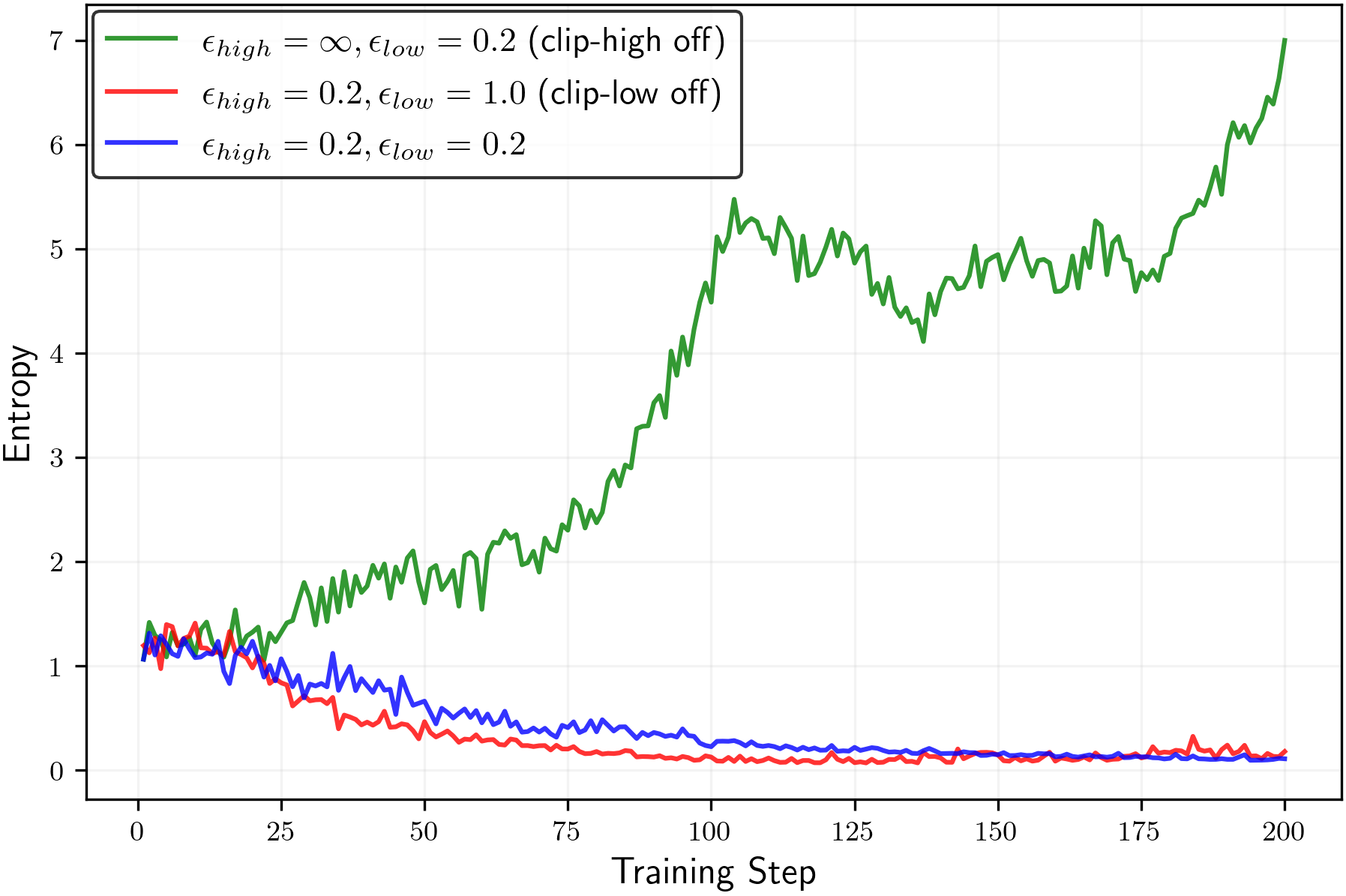

(b)(b)

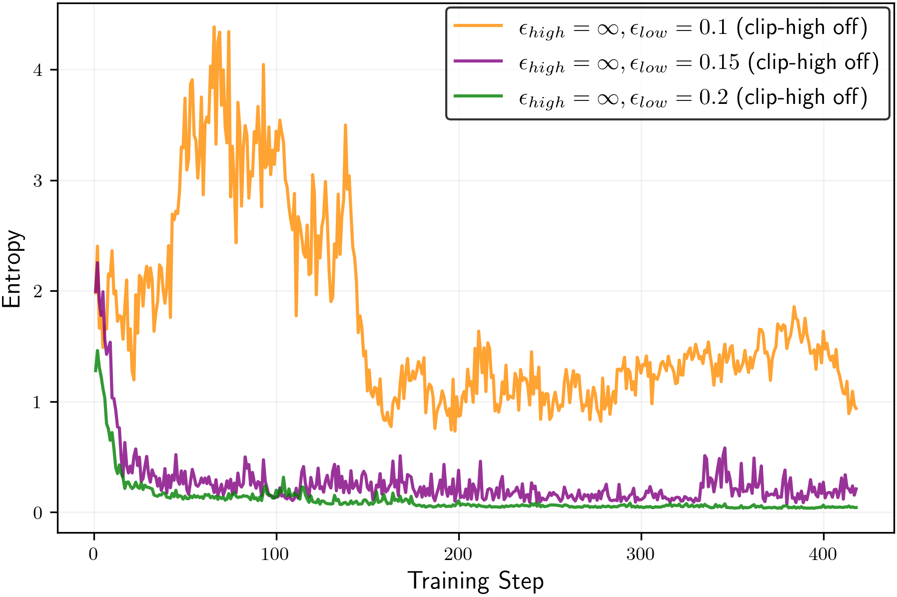
Figure 8:Main experimental results withLlamabase models. Policy entropy change during RL training with(a)random rewards forLlama3.2-1B-Instructand(b)general RLVR rewards forLlama3-8B-Instructmodel. For both random and nonrandom rewards, we observe a clear trend of clip-low increasing entropy and clip-high decreasing it.

C.4Additional experiments forDAPO-Math-17ktraining dataset

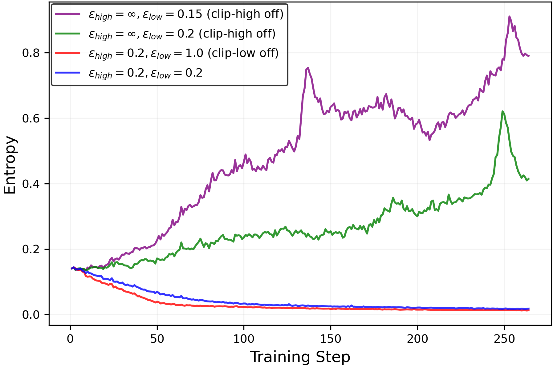Figure 9:Clip ablation study for the entropy dynamics ofQwen2.5-7B-Instructtrained on theDAPO-Math-17kdataset.Here, we present additional experimental results forQwen2.5-7B-Instructmodel trained with theDAPO-Math-17kdataset. In Figure9, we present the result of the clipping ablation experiment observing the entropy dynamics. As expected, we can clearly observe the clipping bias on entropy. In Figure10, we further provide the validation results for themean@32andpass@32metric. Similar to other validation benchmark, deliberate clipping for increased policy entropy effectively hinders exploration degradation throughout the training.

(a)AIME 2024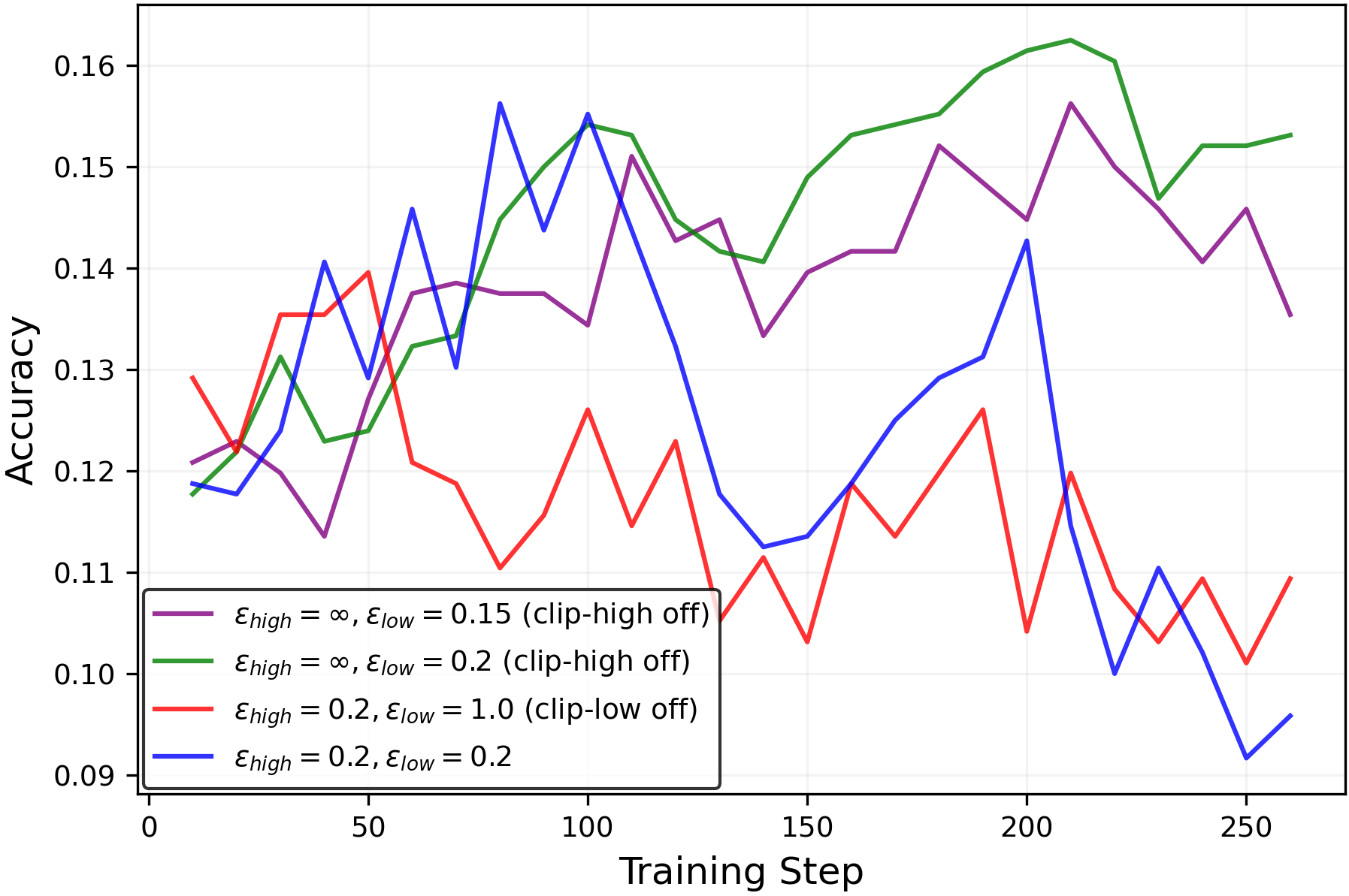

(b)AIME 2025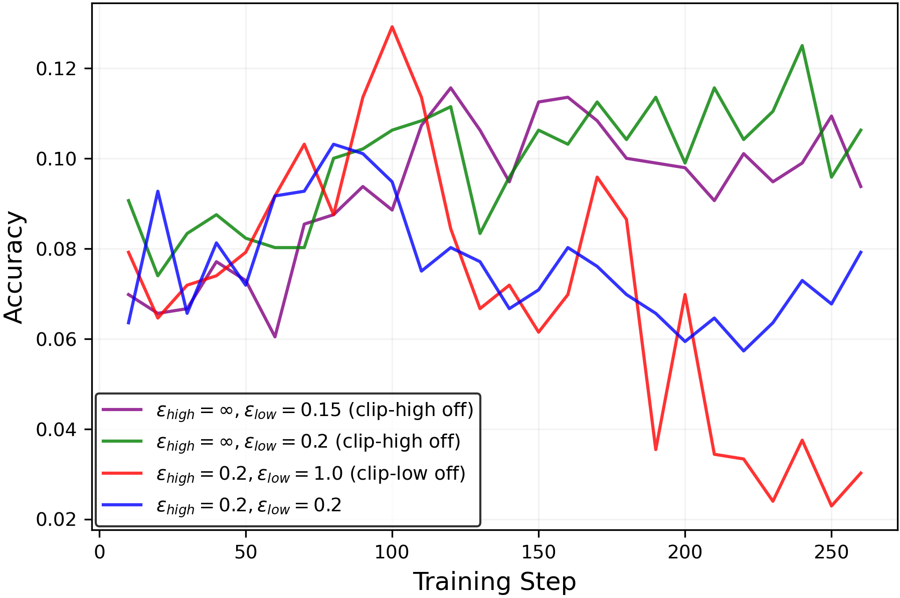

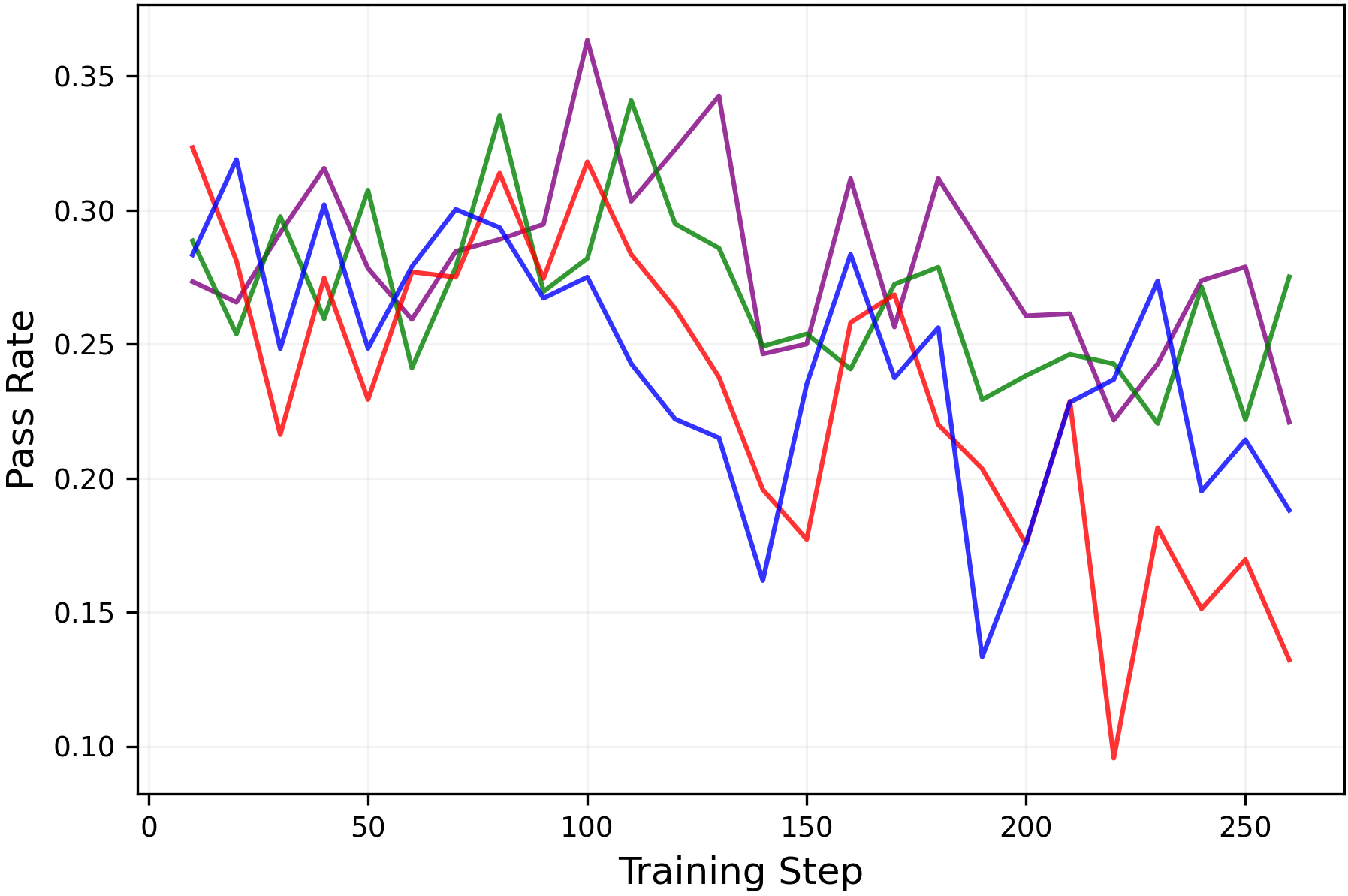
Figure 10:Performance measured by themean@32metric(left)andpass@32metric(right)metric during RLVR for theQwen2.5-7B-Instructmodel trained withDAPO-Math-17kdataset, evaluated on theAIME 2024andAIME 2025datasets.