Diagrams for Penrose Tiles

# Diagrams for Penrose Tiles Source: [https://readerunner.wordpress.com/2021/09/13/diagrams-for-penrose-tiles/](https://readerunner.wordpress.com/2021/09/13/diagrams-for-penrose-tiles/) *Update June 2026*This blog is about drawing finite regions of the infinite non\-periodic tessellations of Roger Penrose’s kite and dart tiles\. It was first written before developing a Haskell package \(PenroseKiteDart\) now available on Hackage\. More info and developments can be seen at the end\. I have made small updates to this blog to keep it compatible with later developments \(and it is no longer a complete literate Haskell file\)\. ## Introduction As part of a collaboration with Stephen Huggett, working on some mathematical properties of Penrose tilings, I recognised the need for quick renderings of tilings\. I thought*Haskell diagrams*would be helpful here, and that turned out to be an excellent choice\. Two dimensional vectors were well\-suited to describing tiling operations and these are included as part of the diagrams package\. The Haskell below uses the Haskell Diagrams package to draw tilings with kites and darts\. It also implements`compChoices`and`decompPatch`which are used for constructing tilings \(explained below\)\. Firstly, these 5 lines are needed in Haskell to use the diagrams package: ``` {-# LANGUAGE NoMonomorphismRestriction #-} {-# LANGUAGE FlexibleContexts #-} {-# LANGUAGE TypeFamilies #-} import Diagrams.Prelude import Diagrams.Backend.SVG.CmdLine ``` and we will also import a module for half tiles \(explained later\) ``` import HalfTile ``` ## Legal tilings These are the kite and dart tiles\. The red line marking here on the right hand copies, is purely to illustrate rules about how tiles can be put together for legal \(non\-periodic\) tilings\. Obviously edges can only be put together when they have the same length\. If all the tiles are marked with red lines as illustrated on the right, the vertices where tiles meet must all have a red line or none must have a red line at that vertex\. This prevents us from forming a simple rombus by placing a kite top at the base of a dart and thus enabling periodic tilings\. All edges are powers of the golden sectionwhich we write as`phi`\. ``` phi :: Double phi = (1.0 + sqrt 5.0) / 2.0 ``` So if the shorter edges are unit length, then the longer edges have length`phi`\. We also have the interesting property of the golden section that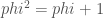and so ,and\. All angles in the figures are multiples of`tt`which is`36 deg`or`1/10 turn`\. We use`ttangle`to express such angles \(e\.g 180 degrees is`ttangle 5`\)\. ``` ttangle:: Int -> Angle Double ttangle n = (fromIntegral (n `mod` 10))*^tt where tt = 1/10 @@ turn ``` ## Pieces In order to implement`compChoices`and`decompPatch`, we need to work with half tiles\. We now define these in the separately imported module`HalfTile`with constructors for Left Dart, Right Dart, Left Kite, Right Kite ``` data HalfTile rep -- defined in HalfTile module = LD rep | RD rep | LK rep | RK rep ``` where`rep`is a type variable allowing for different representations\. However, here, we want to use a more specific type which we call`Piece`\. ``` type Piece = HalfTile [V2 Double] ``` Here the half tiles have a simple 2D vector representation to provide orientation and scale\. \(*Update 2026*: Originally a single vector was used to represent the join edge of a half tile but now we use a list of two vectors instead\)\. The list of two two\-dimensional vectors represents two edges of the half tile \(excluding the*join*edge where half tiles come together\)\. The origin for a dart is the tip, and the origin for a kite is the acute angle tip \(marked in the figure with a red dot\)\. These are the only 4 pieces we use\. They are defined oriented with the join along the x axis\. In the figure they are rotated 90 degrees so the join edges are vertical \(and they have also been labelled\)\. ``` ldart,rdart,lkite,rkite:: Piece ldart = LD [v',v ^-^ v'] where v = unitX v' = phi*^rotate (ttangle 9) v rdart = RD [v',v ^-^ v'] where v = unitX v' = phi*^rotate (ttangle 1) v lkite = LK [v',v ^-^ v'] where v = phi*^unitX v' = rotate (ttangle 1) v rkite = RK [v',v ^-^ v'] where v = phi*^unitX v' = rotate (ttangle 9) v ``` Perhaps confusingly, we regard left and right of a dart differently from left and right of a kite when viewed from the origin\. The diagram shows the right dart before the left dart and the left kite before the right kite\. Thus in a complete tile, going clockwise round the origin the right dart comes before the left dart, but the left kite comes before the right kite\. When it comes to drawing pieces, for the simplest case, we just want to draw the two tile edges of each piece \(and not the join edge\)\. These are the`drawnEdges`of the tile\. We can also use the`joinVector`of the tile \(which is simply the vector sum of the drawn edges\) The drawnEdges are ordered starting from the origin of each piece\. ``` drawnEdges :: Piece -> [V2 Double] joinVector :: Piece -> V2 Double ``` Now drawing lines for the 2 outer edges of a piece we have ``` drawPiece:: Piece -> Diagram B drawPiece = strokeLine . fromOffsets . drawnEdges ``` or just the join edge ``` drawJoin :: Piece -> Diagram B drawJoin piece = strokeLine $ fromOffsets [joinVector piece] ``` or drawing all 3 edges round a piece ``` drawRoundPiece:: Piece -> Diagram B drawRoundPiece = strokeLoop . closeLine . fromOffsets . drawnEdges ``` Sometimes we want two drawn edges but a faint dashed line for the join ``` drawjPiece :: Piece -> Diagram B drawjPiece = drawPiece <> (lw ultraThin . joinDashing . drawJoin) where joinDashing = normalized 0.003 `atLeast` output 1.0 ``` To fill half tile pieces, we can use`fillOnlyPiece`which fills without showing edges of a half tile \(by using line width none\)\. ``` fillOnlyPiece:: Colour Double -> Piece -> Diagram B fillOnlyPiece col piece = drawRoundPiece piece # fc col # lw none ``` We also use`fillPieceDK`which fills darts and kites with given colours and also draws edges using drawPiece\. ``` fillPieceDK:: Colour Double -> Colour Double -> Piece -> Diagram B fillPieceDK dcol kcol piece = drawPiece piece <> fillOnlyPiece col piece where col = case piece of (LD _) -> dcol (RD _) -> dcol (LK _) -> kcol (RK _) -> kcol ``` For an alternative fill operation on whole tiles, we calculated a list of the 4 tile edges of a completed half\-tile piece clockwise from the origin of the tile\. This allows colour filling a whole tile, but it does rely on prior transformations preserving angles as it uses angles in the definition \(not shown\)\. ``` wholeTileEdges:: Piece -> [V2 Double] ``` To fill whole tiles with colours, darts with`dcol`and kites with`kcol`we can now use`leftFillPieceDK`\. This uses only the left pieces to identify the whole tile and ignores right pieces so that a tile is not filled twice and uses`wholeTileEdges`\. ``` leftFillPieceDK:: Colour Double -> Colour Double -> Piece -> Diagram B leftFillPieceDK dcol kcol c = case c of (LD _) -> (strokeLoop $ glueLine $ fromOffsets $ wholeTileEdges c) # fc dcol (LK _) -> (strokeLoop $ glueLine $ fromOffsets $ wholeTileEdges c) # fc kcol _ -> mempty ``` By making`Pieces`transformable we can reuse generic transform operations\. These 4 lines of code are required to do this ``` type instance N (HalfTile a) = N a type instance V (HalfTile a) = V a instance Transformable a => Transformable (HalfTile a) where transform t ht = fmap (transform t) ht ``` So we can scale and rotate a piece by an angle \(positive rotations are in the anticlockwise direction\) but we cannote translate until they are located \(as Patches\)\. ``` scale :: Double -> Piece -> Piece rotate :: Angle Double -> Piece -> Piece ``` ## Patches A patch is a list of located pieces \(each with a 2D point\) ``` type Patch = [Located Piece] ``` To turn a whole patch into a diagram using some function`pd`for drawing the pieces, we use`drawWith` ``` class Drawable a where drawWith :: (Piece -> Diagram B) -> a -> Diagram B instance Drawable Patch where drawWith pd = position $ fmap (viewLoc . mapLoc pd) ``` Here`mapLoc`applies a function to the piece in a located piece – producing a located diagram in this case, and`viewLoc`returns the pair of point and diagram from a located diagram\. Finally`position`forms a single diagram from the list of pairs of points and diagrams\. \(The use of a class definition here anticipates more instances in later developments\)\. We now define the most common special cases: ``` draw :: Drawable a => a -> Diagram B draw = drawWith drawPiece drawj :: Drawable a => a -> Diagram B drawj = drawWith drawjPiece fillDK:: Drawable a => Colour Double -> Colour Double -> a -> Diagram B fillDK c1 c2 = drawWith (fillPieceDK c1 c2) ``` Patches are automatically inferred to be transformable, so we can also scale a patch, translate a patch by a vector, and rotate a patch by an angle \(for example\)\. ``` scale :: Double -> Patch -> Patch rotate :: Angle Double -> Patch -> Patch translate :: V2 Double -> Patch -> Patch ``` As an aid to creating patches with 5\-fold rotational symmetry, we combine 5 copies of a basic patch \(rotated by multiples of`ttangle 2`successively\)\. ``` penta:: Patch -> Patch penta p = concatMap copy [0..4] where copy n = rotate (ttangle (2*n)) p ``` This must be used with care to avoid nonsense patches\. But two special cases are ``` sun,star :: Patch sun = penta [rkite `at` origin, lkite `at` origin] star = penta [rdart `at` origin, ldart `at` origin] ``` This figure shows some example patches, drawn with`draw`The first is a`star`and the second is a`sun`\. The tools so far for creating patches may seem limited \(and do not help with ensuring legal tilings\), but there is an even bigger problem\. ## Correct Tilings Unfortunately, correct tilings – that is, tilings which can be extended to infinity – are not as simple as just legal tilings\. It is not enough to have a legal tiling, because an apparent \(legal\) choice of placing one tile can have non\-local consequences, causing a conflict with a choice made far away in a patch of tiles, resulting in a patch which cannot be extended\. This suggests that constructing correct patches is far from trivial\. The infinite number of possible infinite tilings do have some remarkable properties\. Any finite patch from one of them, will occur in all the others \(infinitely many times\) and within a relatively small radius of any point in an infinite tiling\. \(For details of this see links at the end\)\. This is why we need a different approach to constructing larger patches\. There are two significant processes used for creating patches, namely`inflate`\(also called*compose*\) and`decompose`\. To understand these processes, take a look at the following figure\. Here the*small*pieces have been drawn in an unusual way\. The edges have been drawn with dashed lines, but long edges of kites have been emphasised with a solid line and the join edges of darts marked with a red line\. From this you may be able to make out a patch of larger scale kites and darts\. This is an inflated patch arising from the smaller scale patch\. Conversely, the larger kites and darts decompose to the smaller scale ones\. ## Decomposition Since the rule for decomposition is uniquely determined, we can express it as a simple function on patches\. ``` decompPatch :: Patch -> Patch decompPatch = concatMap decompPiece ``` where the function`decompPiece`acts on located pieces and produces a list of the smaller located pieces contained in the piece\. For example, a larger right dart will produce both a smaller right dart and a smaller left kite\. Decomposing a located piece also takes care of the location, scale and rotation of the new pieces\. \(*Revised version 2026 avoiding use of angles*\)\. ``` decompPiece :: Located Piece -> [Located Piece] decompPiece lp = case viewLoc lp of (p, RD [z1,z2])-> [ LK [s1, s2 ] `at` p , RD [z2, negate s2] `at` (p .+^ z1) ] where s1 = (phi-1) *^ z1 s2 = sumV [z1,z2] ^-^ s1 (p, LD [z1,z2])-> [ RK [s1, s2 ] `at` p , LD [z2, negate s2] `at` (p .+^ z1) ] where s1 = (phi-1) *^ z1 s2 = sumV [z1,z2] ^-^ s1 (p, RK [z1,z2])-> [ RD [s1, s2] `at` p , LK [s4, negate s2] `at` (p .+^ z1) , RK [z2, s3] `at` (p .+^ z1) ] where j = sumV [z1,z2] s1 = (phi-1) *^ j s2 = (2-phi) *^ z1 ^-^ s1 s3 = (phi-2) *^ j s4 = (1-phi) *^ z1 (p, LK [z1,z2])-> [ LD [s1, s2] `at` p , RK [s4, negate s2] `at` (p .+^ z1) , LK [z2, s3] `at` (p .+^ z1) ] where j = sumV [z1,z2] s1 = (phi-1) *^ j s2 = (2-phi) *^ z1 ^-^ s1 s3 = (phi-2) *^ j s4 = (1-phi) *^ z1 other -> error $ "decompPiece: " ++ show other ++ "/n" ``` This is illustrated in the following figure for the cases of a right dart and a right kite\. The symmetric diagrams for left pieces are easy to work out from these, so they are not illustrated\. With the`decompPatch`operation we can start with a simple correct patch, and decompose repeatedly to get more and more detailed patches\. \(Each decomposition scales the tiles down by a factor ofbut we can rescale at any time\.\) This figure illustrates how each piece decomposes with 4 decomposition steps below each one\. ``` thePieces = [ldart, rdart, lkite, rkite] fourDecomps = hsep 1 $ fmap decomps thePieces # lw thin where decomps pc = vsep 1 $ fmap drawj $ take 5 $ decompositionsP [pc `at` origin] ``` We have made use of the fact that we can create an infinite list of finer and finer decompositions of any patch, using: ``` decompositionsP:: Patch -> [Patch] decompositionsP = iterate decompPatch ``` We could get the n\-fold decomposition of a patch as just the nth item in a list of decompositions\. For example, here is an infinite list of decomposed versions of`sun`\. ``` suns = decompositionsP sun ``` The coloured tiling shown at the beginning is simply 6 decompositions of`sun`displayed using`leftFillPieceDK` ``` leftFilledSun6 :: Diagram B leftFilledSun6 = drawWith (leftFillPieceDK red darkviolet) sun6 # lw thin ``` The earlier figure illustrating larger kites and darts emphasised from the smaller ones is also`suns\!\!6`but this time pieces are drawn with`experiment`\. ``` experimentFig = drawWith experiment (suns!!6) # lw thin experiment:: Piece -> Diagram B experiment pc = emph pc <> (drawRoundPiece pc # dashingN [0.002,0.002] 0 # lw ultraThin) where emph pc = case pc of (LD v) -> (strokeLine . fromOffsets) [v] # lc red -- emphasise join edge of darts in red (RD v) -> (strokeLine . fromOffsets) [v] # lc red (LK v) -> (strokeLine . fromOffsets) [rotate (ttangle 1) v] -- emphasise long edge for kites (RK v) -> (strokeLine . fromOffsets) [rotate (ttangle 9) v] ``` ## Compose Choices You might expect composition \(also called*inflation*\) to be a kind of inverse to decomposition, but it is a bit more complicated than that\. With our current representation of pieces, we can only compose single pieces\. This amounts to embedding the piece into a larger piece that matches how the larger piece decomposes\. There is thus a choice at each composition step as to which of several possibilities we select as the larger half\-tile\. We represent this choice as a list of alternatives\. This list should not be confused with a Patch\. It only makes sense to select one of the alternatives giving a new single piece\. The earlier diagram illustrating how decompositions are calculated also shows the two choices for embedding a right dart into either a right kite or a larger right dart\. There will be two symmetric choices for a left dart, and three choices for left and right kites\. Once again we work with located pieces to ensure the resulting larger piece contains the original in its original position in a decomposition\. \(*Revised version 2026 avoiding use of angles*\)\. ``` compChoices :: Located Piece -> [Located Piece] compChoices lp = case viewLoc lp of (p, RD [s1,s2])-> [ RD [negate z1,s1] `at` (p .+^ z1) , RK [z1, z2] `at` p ] where z1 = (phi+1) *^ sumV [s1,s2] z2 = phi *^ s1 ^-^ z1 (p, LD [s1,s2])-> [ LD [negate z1,s1] `at` (p .+^ z1) , LK [z1, z2] `at` p ] where z1 = (phi+1) *^ sumV [s1,s2] z2 = phi *^ s1 ^-^ z1 (p, RK [s1,s2])-> [ LD [z1, z2] `at` p , LK [negate z1,z3] `at` (p .+^ z1) , RK [negate z,s1] `at` (p .+^ z) ] where z1 = phi *^ s1 z = s1 ^+^ (phi+1) *^ s2 z2 = sumV [s1,s2] ^-^ z1 z3 = z1 ^+^ phi *^ z2 (p, LK [s1,s2])-> [ RD [z1, z2] `at` p , RK [negate z1,z3] `at` (p .+^ z1) , LK [negate z,s1] `at` (p .+^ z) ] where z1 = phi *^ s1 z = s1 ^+^ (phi+1) *^ s2 z2 = sumV [s1,s2] ^-^ z1 z3 = z1 ^+^ phi *^ z2 other -> error $ "compChoices: " ++ show other ++ "/n" ``` As the result is a list of alternatives, we need to select one to do further inflations\. We can express all the alternatives after n steps as`compNChoices n`where ``` compNChoices :: Int -> Located Piece -> [Located Piece] compNChoices 0 lp = [lp] compNChoices n lp = do lp' <- inflate lp inflations (n-1) lp' ``` This figure illustrates 5 consecutive choices for composing a left dart to produce a left kite\. On the left, the finishing piece is shown with the starting piece embedded, and on the right the 5\-fold decomposition of the result is shown\. ``` fiveCompChoices = hsep 1 $ [ draw [ld] <> draw [lk'] , draw (decompositionsP [lk'] !!5) ] where ld = (ldart `at` origin) lk = compChoices ld !!1 rk = compChoices lk !!1 rk' = compChoices rk !!2 ld' = compChoices rk' !!0 lk' = compChoices ld' !!1 ``` Finally, at the end of this haskell program we choose which figure to draw as output\. ``` fig :: Diagram B fig = leftFilledSun6 main = mainWith fig ``` That’s it\. But,*What about composing whole patches?*, I hear you ask\. Unfortunately we need to answer questions like what pieces are adjacent to a piece in a patch and whether there is a corresponding other half for a piece\. These cannot be done with our simple vector representations\. We would need some form of planar graph representation, which is much more involved\. That is another story which can be found in these subsequent blogs\. - [Graphs, Kites and Darts](https://readerunner.wordpress.com/2022/01/06/graphs-kites-and-darts/)intoduced Tgraphs\. This gave more details of implementation and results of early explorations\. \(The class`Forcible`was introduced subsequently\)\. - [Empires and SuperForce](https://readerunner.wordpress.com/2023/04/26/graphs-kites-and-darts-empires-and-superforce/)– these new operations were based on observing properties of boundaries of forced Tgraphs\. - [Graphs,Kites and Darts and Theorems](https://readerunner.wordpress.com/2023/09/12/graphs-kites-and-darts-and-theorems/)established some important results relating`force`,`compose`,`decompose`\. - [PenroseKiteDart User Guide](https://readerunner.wordpress.com/2024/04/08/penrosekitedart-user-guides/)for the PenroseKiteDart package\. Source code for library version of the above code \(as part of the PenroseKiteDart package on[Hackage](https://hackage.haskell.org/package/PenroseKiteDart)\) can be seen at[GitHub](https://github.com/chrisreade/PenroseKiteDart)\. Many thanks to Stephen Huggett for his inspirations concerning the tilings\. ## Further reading on Penrose Tilings As well as the Wikipedia entry[Penrose Tilings](https://en.wikipedia.org/wiki/Penrose_tiling)I recommend two articles in Scientific American from 2005 by David Austin[Penrose Tiles Talk Across Miles](http://www.ams.org/publicoutreach/feature-column/fcarc-penrose)and[Penrose Tilings Tied up in Ribbons](http://www.ams.org/publicoutreach/feature-column/fcarc-ribbons)\. There is also a very interesting article by Roger Penrose himself: Penrose R*Tilings and quasi\-crystals; a non\-local growth problem?*in Aperiodicity and Order 2, edited by Jarich M, Academic Press, 1989\. More information about the diagrams package can be found from the home page[Haskell diagrams](https://diagrams.github.io/)