This article explains Behavioral Cloning, an imitation learning technique used to train policies from expert demonstrations, discussing its theoretical basis in maximum likelihood estimation and its historical applications like AlphaGo.
<p><em>By Surya Vengadesan</em></p><h2>Introduction</h2><p>In this blog post, we will be covering imitation learning, reinforcement learning’s sibling. While the goal of reinforcement learning is to cleverly solve a policy given an MDP that models an environment (see <a href="https://ml.berkeley.edu/blog/posts/mdps/">prev. post</a>), the goal of Imitation Learning is to learn a policy given just trajectories of an agent within the MDP. In particular, we will be covering a specific algorithm called Behavioral Cloning (BC), which was employed to train self-driving vehicles all the way back in the <a href="https://papers.nips.cc/paper/1988/file/812b4ba287f5ee0bc9d43bbf5bbe87fb-Paper.pdf">1980’s</a>, and was used in the first implementation of <a href="https://www.nature.com/articles/nature16961">Alpha-Go</a>. If you are unfamiliar with RL and MDP’s, don’t worry, that information can be abstracted away for understanding the ideas below.</p><h2>Behavioral Cloning</h2><p>The main idea behind Behavioral Cloning is to learn a policy for an MDP given expert demonstrations. For example, you might collect a dataset of someone’s steering directions given an image from a car to learn a policy that can do rudimentary self driving. This policy is simply a function that maps a set of states to a distribution over actions. The natural question to ask is, how does one construct such an algorithm? In this blog post, we will cover the required theory, then proceed to layout the building blocks of a BC algorithm and implement it inside an OpenAI gym environment.</p><div class="captioned-image-container"><figure><a class="image-link image2 is-viewable-img" target="_blank" href="https://substackcdn.com/image/fetch/$s_!ODkg!,f_auto,q_auto:good,fl_progressive:steep/https%3A%2F%2Fsubstack-post-media.s3.amazonaws.com%2Fpublic%2Fimages%2Fd68dba66-a50b-434b-a189-d001df3eb23c_598x333.png" data-component-name="Image2ToDOM"><div class="image2-inset"><picture><source type="image/webp" srcset="https://substackcdn.com/image/fetch/$s_!ODkg!,w_424,c_limit,f_webp,q_auto:good,fl_progressive:steep/https%3A%2F%2Fsubstack-post-media.s3.amazonaws.com%2Fpublic%2Fimages%2Fd68dba66-a50b-434b-a189-d001df3eb23c_598x333.png 424w, https://substackcdn.com/image/fetch/$s_!ODkg!,w_848,c_limit,f_webp,q_auto:good,fl_progressive:steep/https%3A%2F%2Fsubstack-post-media.s3.amazonaws.com%2Fpublic%2Fimages%2Fd68dba66-a50b-434b-a189-d001df3eb23c_598x333.png 848w, https://substackcdn.com/image/fetch/$s_!ODkg!,w_1272,c_limit,f_webp,q_auto:good,fl_progressive:steep/https%3A%2F%2Fsubstack-post-media.s3.amazonaws.com%2Fpublic%2Fimages%2Fd68dba66-a50b-434b-a189-d001df3eb23c_598x333.png 1272w, https://substackcdn.com/image/fetch/$s_!ODkg!,w_1456,c_limit,f_webp,q_auto:good,fl_progressive:steep/https%3A%2F%2Fsubstack-post-media.s3.amazonaws.com%2Fpublic%2Fimages%2Fd68dba66-a50b-434b-a189-d001df3eb23c_598x333.png 1456w" sizes="100vw"><img src="https://substackcdn.com/image/fetch/$s_!ODkg!,w_1456,c_limit,f_auto,q_auto:good,fl_progressive:steep/https%3A%2F%2Fsubstack-post-media.s3.amazonaws.com%2Fpublic%2Fimages%2Fd68dba66-a50b-434b-a189-d001df3eb23c_598x333.png" width="598" height="333" data-attrs="{"src":"https://substack-post-media.s3.amazonaws.com/public/images/d68dba66-a50b-434b-a189-d001df3eb23c_598x333.png","srcNoWatermark":null,"fullscreen":null,"imageSize":null,"height":333,"width":598,"resizeWidth":null,"bytes":null,"alt":null,"title":null,"type":null,"href":null,"belowTheFold":false,"topImage":true,"internalRedirect":null,"isProcessing":false,"align":null,"offset":false}" class="sizing-normal" alt="" srcset="https://substackcdn.com/image/fetch/$s_!ODkg!,w_424,c_limit,f_auto,q_auto:good,fl_progressive:steep/https%3A%2F%2Fsubstack-post-media.s3.amazonaws.com%2Fpublic%2Fimages%2Fd68dba66-a50b-434b-a189-d001df3eb23c_598x333.png 424w, https://substackcdn.com/image/fetch/$s_!ODkg!,w_848,c_limit,f_auto,q_auto:good,fl_progressive:steep/https%3A%2F%2Fsubstack-post-media.s3.amazonaws.com%2Fpublic%2Fimages%2Fd68dba66-a50b-434b-a189-d001df3eb23c_598x333.png 848w, https://substackcdn.com/image/fetch/$s_!ODkg!,w_1272,c_limit,f_auto,q_auto:good,fl_progressive:steep/https%3A%2F%2Fsubstack-post-media.s3.amazonaws.com%2Fpublic%2Fimages%2Fd68dba66-a50b-434b-a189-d001df3eb23c_598x333.png 1272w, https://substackcdn.com/image/fetch/$s_!ODkg!,w_1456,c_limit,f_auto,q_auto:good,fl_progressive:steep/https%3A%2F%2Fsubstack-post-media.s3.amazonaws.com%2Fpublic%2Fimages%2Fd68dba66-a50b-434b-a189-d001df3eb23c_598x333.png 1456w" sizes="100vw" fetchpriority="high"></picture><div class="image-link-expand"><div class="pencraft pc-display-flex pc-gap-8 pc-reset"><button tabindex="0" type="button" class="pencraft pc-reset pencraft icon-container restack-image"><svg role="img" width="20" height="20" viewBox="0 0 20 20" fill="none" stroke-width="1.5" stroke="var(--color-fg-primary)" stroke-linecap="round" stroke-linejoin="round" xmlns="http://www.w3.org/2000/svg"><g><title></title><path d="M2.53001 7.81595C3.49179 4.73911 6.43281 2.5 9.91173 2.5C13.1684 2.5 15.9537 4.46214 17.0852 7.23684L17.6179 8.67647M17.6179 8.67647L18.5002 4.26471M17.6179 8.67647L13.6473 6.91176M17.4995 12.1841C16.5378 15.2609 13.5967 17.5 10.1178 17.5C6.86118 17.5 4.07589 15.5379 2.94432 12.7632L2.41165 11.3235M2.41165 11.3235L1.5293 15.7353M2.41165 11.3235L6.38224 13.0882"></path></g></svg></button><button tabindex="0" type="button" class="pencraft pc-reset pencraft icon-container view-image"><svg xmlns="http://www.w3.org/2000/svg" width="20" height="20" viewBox="0 0 24 24" fill="none" stroke="currentColor" stroke-width="2" stroke-linecap="round" stroke-linejoin="round" class="lucide lucide-maximize2 lucide-maximize-2"><polyline points="15 3 21 3 21 9"></polyline><polyline points="9 21 3 21 3 15"></polyline><line x1="21" x2="14" y1="3" y2="10"></line><line x1="3" x2="10" y1="21" y2="14"></line></svg></button></div></div></div></a></figure></div><p>In order to best fit a policy with demonstrations, we first need to introduce the concept of <a href="https://en.wikipedia.org/wiki/Likelihood_function">likelihood</a>. In short, for those familiar with statistical inference, BC performs maximum likelihood estimation. We want to estimate the parameters of a model that best fits to demonstrations, by assigning high likelihoods to the demonstrations under the learned policy.</p><h2>MLE on Buffon’s Needle</h2><p>What does it mean to maximize likelihood? While a probability maps some event to a chance of it occurring, a likelihood maps a model parameter to the joint probability of a set of observations. To solidify this defintion, let’s perform maximum likelihood estimation on a common probability problem — Buffon’s Needle.</p><div class="captioned-image-container"><figure><a class="image-link image2" target="_blank" href="https://substackcdn.com/image/fetch/$s_!uck-!,f_auto,q_auto:good,fl_progressive:steep/https%3A%2F%2Fsubstack-post-media.s3.amazonaws.com%2Fpublic%2Fimages%2F0255c3b4-9cfc-45d5-8e72-ae7ba9c2911f_241x218.png" data-component-name="Image2ToDOM"><div class="image2-inset"><picture><source type="image/webp" srcset="https://substackcdn.com/image/fetch/$s_!uck-!,w_424,c_limit,f_webp,q_auto:good,fl_progressive:steep/https%3A%2F%2Fsubstack-post-media.s3.amazonaws.com%2Fpublic%2Fimages%2F0255c3b4-9cfc-45d5-8e72-ae7ba9c2911f_241x218.png 424w, https://substackcdn.com/image/fetch/$s_!uck-!,w_848,c_limit,f_webp,q_auto:good,fl_progressive:steep/https%3A%2F%2Fsubstack-post-media.s3.amazonaws.com%2Fpublic%2Fimages%2F0255c3b4-9cfc-45d5-8e72-ae7ba9c2911f_241x218.png 848w, https://substackcdn.com/image/fetch/$s_!uck-!,w_1272,c_limit,f_webp,q_auto:good,fl_progressive:steep/https%3A%2F%2Fsubstack-post-media.s3.amazonaws.com%2Fpublic%2Fimages%2F0255c3b4-9cfc-45d5-8e72-ae7ba9c2911f_241x218.png 1272w, https://substackcdn.com/image/fetch/$s_!uck-!,w_1456,c_limit,f_webp,q_auto:good,fl_progressive:steep/https%3A%2F%2Fsubstack-post-media.s3.amazonaws.com%2Fpublic%2Fimages%2F0255c3b4-9cfc-45d5-8e72-ae7ba9c2911f_241x218.png 1456w" sizes="100vw"><img src="https://substackcdn.com/image/fetch/$s_!uck-!,w_1456,c_limit,f_auto,q_auto:good,fl_progressive:steep/https%3A%2F%2Fsubstack-post-media.s3.amazonaws.com%2Fpublic%2Fimages%2F0255c3b4-9cfc-45d5-8e72-ae7ba9c2911f_241x218.png" width="241" height="218" data-attrs="{"src":"https://substack-post-media.s3.amazonaws.com/public/images/0255c3b4-9cfc-45d5-8e72-ae7ba9c2911f_241x218.png","srcNoWatermark":null,"fullscreen":null,"imageSize":null,"height":218,"width":241,"resizeWidth":null,"bytes":null,"alt":null,"title":null,"type":null,"href":null,"belowTheFold":true,"topImage":false,"internalRedirect":null,"isProcessing":false,"align":null,"offset":false}" class="sizing-normal" alt="" srcset="https://substackcdn.com/image/fetch/$s_!uck-!,w_424,c_limit,f_auto,q_auto:good,fl_progressive:steep/https%3A%2F%2Fsubstack-post-media.s3.amazonaws.com%2Fpublic%2Fimages%2F0255c3b4-9cfc-45d5-8e72-ae7ba9c2911f_241x218.png 424w, https://substackcdn.com/image/fetch/$s_!uck-!,w_848,c_limit,f_auto,q_auto:good,fl_progressive:steep/https%3A%2F%2Fsubstack-post-media.s3.amazonaws.com%2Fpublic%2Fimages%2F0255c3b4-9cfc-45d5-8e72-ae7ba9c2911f_241x218.png 848w, https://substackcdn.com/image/fetch/$s_!uck-!,w_1272,c_limit,f_auto,q_auto:good,fl_progressive:steep/https%3A%2F%2Fsubstack-post-media.s3.amazonaws.com%2Fpublic%2Fimages%2F0255c3b4-9cfc-45d5-8e72-ae7ba9c2911f_241x218.png 1272w, https://substackcdn.com/image/fetch/$s_!uck-!,w_1456,c_limit,f_auto,q_auto:good,fl_progressive:steep/https%3A%2F%2Fsubstack-post-media.s3.amazonaws.com%2Fpublic%2Fimages%2F0255c3b4-9cfc-45d5-8e72-ae7ba9c2911f_241x218.png 1456w" sizes="100vw" loading="lazy"></picture><div></div></div></a></figure></div><p>Given a set of parallel lines equally separated by distance <em>d</em>, you randomly drop the needle of length lll between the lines, what’s the probability that the needle touches the lines. The parameters here are <em>{l,d}</em>, which we can attempt to estimate given some sample droppings. Formally, if we define <em>x</em> to be the distance from the midpoint of a needle to the closest line, and <em>θ</em> to to be the angle of intersection as defined above, we get the nice uniform probability distributiondefined by Buffon, a French naturalist.</p><div class="latex-rendered" data-attrs="{"persistentExpression":"P(\\text{Needle touches a line } | X = x, \\Theta = \\theta) = \\frac{2l}{\\pi d}","id":"XCZNYMGUJL"}" data-component-name="LatexBlockToDOM"></div><p>Assume we fix the distance between two parallel lines to <em>d=3</em>, and assume we are given trial datapoints of a needle dropped three times, each time touching a line: </p><div class="latex-rendered" data-attrs="{"persistentExpression":"\\mathcal{D} = \\{d_1, d_2, d_3\\} = \\{(0, 0), (1, \\frac{\\pi}{2}), (1, \\frac{\\pi}{6})\\}","id":"KIBWUDQBPR"}" data-component-name="LatexBlockToDOM"></div><p>What length <em>l</em> parameter will maxmize the likelihood of recreating this dataset? Given that likelihood is defined as the product of the probabilites of the observations occuring we have the following form:</p><div class="latex-rendered" data-attrs="{"persistentExpression":"\\mathcal{L}(\\mathcal{D}|l) = \\Pi_{i=1}^3 P(d_i)","id":"MDXGYZALCR"}" data-component-name="LatexBlockToDOM"></div><p>To solve for this specific example, we can first find the boundaries of the parameter and choose one that maximizes the likelihood function above. The first boundary is that <em>l<d</em> so a needle cannot intersect more than one line at a time. Also, by the geometry of the problem, the needle intersects when </p><div class="latex-rendered" data-attrs="{"persistentExpression":"x < \\frac{l}{2} sin(\\theta)","id":"BEETXGUETN"}" data-component-name="LatexBlockToDOM"></div><p>which gives us three additional inequalities. </p><div class="latex-rendered" data-attrs="{"persistentExpression":"0 \\leq \\frac{l}{2} * 0","id":"HSHXPZNTAJ"}" data-component-name="LatexBlockToDOM"></div><div class="latex-rendered" data-attrs="{"persistentExpression":"1 \\leq \\frac{l}{2} * 1","id":"PTUXXCIQYG"}" data-component-name="LatexBlockToDOM"></div><div class="latex-rendered" data-attrs="{"persistentExpression":"1 \\leq \\frac{l}{2} * \\frac{\\sqrt{3}}{2}","id":"LSGDMBPTXW"}" data-component-name="LatexBlockToDOM"></div><p>The intersection of all these intervals is </p><div class="latex-rendered" data-attrs="{"persistentExpression":"\\frac{\\sqrt{3}}{2} \\leq l \\leq 3","id":"DENRJLGWEP"}" data-component-name="LatexBlockToDOM"></div><p>Now, </p><div class="latex-rendered" data-attrs="{"persistentExpression":"argmax_{\\frac{\\sqrt{3}}{2} \\leq l \\leq 3} \\mathcal{L}(\\mathcal{D}|l) = 3","id":"RFOOJXVRIV"}" data-component-name="LatexBlockToDOM"></div><div class="latex-rendered" data-attrs="{"persistentExpression":"\\mathcal{L} (\\mathcal{D}|l = 3) = (\\frac{2l}{3\\pi})^3 = \\frac{8}{9\\pi^3}.","id":"MSCSVHUYCZ"}" data-component-name="LatexBlockToDOM"></div><p>We have just shown, that given some observations, we can compute the length of the needle (i.e. <em>l=3</em>) that most likely produced the data. This set of analytic steps to find optimal paramters, is in essence what we do with BC, but on more complex environments where nice steps can no longer be applied.</p><h2>MLE for Policy Estimation</h2><p>Therefore, when applying this technique to the setting of reinforcement learning and control, we can represent an event as a trajectory (i.e. a set of sequential state action pairs) which has a specific probability of occurring given a policy. Below, τ is the trajectory of state action pairs (<em>s<sub>i</sub></em>,<em>a<sub>i</sub></em>), <em>π(a<sub>i</sub>∣s<sub>i</sub>)</em> is the policy’s proability of taking an action <em>a<sub>i</sub></em> given you are in state <em>s<sub>i</sub></em>​, and T(⋅) is the transition proability of ending up in state <em>s<sub>i+1</sub></em>​ given you took the state action pair (<em>s<sub>i</sub></em>,<em>a<sub>i</sub></em>):</p><div class="latex-rendered" data-attrs="{"persistentExpression":"\\tau = \\{(s_0, a_0), (s_1, a_1), \\cdots, (s_n, a_n)\\} ","id":"KGTACGVVUU"}" data-component-name="LatexBlockToDOM"></div><div class="latex-rendered" data-attrs="{"persistentExpression":"P(\\tau) = \\Pi_{i = 0}^{n} \\pi(a_i|s_i)\\mathcal{T}(s_{i+1}|s_i, a_i)","id":"MQSTEKPQLO"}" data-component-name="LatexBlockToDOM"></div><p>Given a dataset of such demonstration trajectories, the likelihood therefore would be the product of all the probabilities of the individual trajectories. The below equation should resemble the example above with Buffon’s needle:</p><div class="latex-rendered" data-attrs="{"persistentExpression":"\\mathcal{D} = \\{\\tau^1, \\cdots , \\tau^n\\}","id":"WQTZGSXKMF"}" data-component-name="LatexBlockToDOM"></div><div class="latex-rendered" data-attrs="{"persistentExpression":"\\mathcal{L}(\\mathcal{D}) = \\Pi_{i = 1}^{n} P(\\tau^i)","id":"YGQNYTPPLE"}" data-component-name="LatexBlockToDOM"></div><p>In order to estimate the parameters for more complex models, we can use supervised learning techniques, such that given a set of input states and output actions, we learn a mapping between the two that serves as the policy. By tuning the parameters of a supervised learning model, we can solve the MLE problem above.</p><p>Therefore, the first step in solving this optimization problem is to pick a specific model to optimize. For example, the model could be some neural network that takes a state as input and outputs an action. The specific neural network architecture you use should be chosen and engineered for your specific task.</p><h2>BC on Cartpole</h2><p>In the remainder of this article, we will put all of these pieces together as we construct a behavioral cloning implementation, using a few barebone methods. Our BC implementation will consist of three components:</p><pre><code>(1) Dataset: Cartpole
(2) Model: FC Neural Network
(3) Loss: Binary Cross entropy Loss</code></pre><p>To demonstrate BC we’ve chosen a simple graphical environment in the Open AI gym, called cartpole. The agent consists of a cart set on a frictionless surface with a frictionless joint that attaches a pole on top. The goal of the agent is to balance this pole. It has a discrete action space: {push to the left - 0, push to the right - 1} and a continuous state space: {cart position - [-4.8, 4.8] , cart velocity - [-inf, inf] , pole angle - [-24, 24 (deg)], pole angular velocity - [-inf, inf]}.</p><p>To obtain expert demostrations, we quickly train Open AI’s PPO implementation and sample from it’s trained agent. Now, we are left with the supervised learning problem which is the crux of BC. We go about solving this supervised learning problem using a fully connected neural net with three layers follow by ReLU nonlinearities and a final sigmoid nonlinearity. Given the training data, we can now approximate a function that maps states to actions, which serves as your behaviorally cloned policy.</p><p>Although our expert PPO agent is familiar with the reward structure of the environment, we can achieve similar performance without knowing the underlying MDP. But, when our trained agent interacts with states not covered by the expert demostrator, it won’t know how to behave. This issue, refered to as distribution shift, can cause a compounding sequence of incorrect steps that wreck havoc. If a BC agent encounters a state that it is even slightly unfamiliar, it will take a wrong action, leading it towards a next state even more unfamiliar — diverging from the expert very easily. When it came to our specific task, we tried our best to engineer around this issue and others that arose — see below.</p><h2>Engineering Choices and Code</h2><p>During the process of training the behavioral cloning net, a few engineering tricks were required to get the clone working, listed below for reference.</p><p>(1) Adding a final sigmoid (i.e. not TanH or ReLU) nonlinearity to account for the binary actions and to avoid numerical instability (2) Generating more sample data from the expert if too few isn’t sufficient enough to cover the intricate expert behavior (3) Not making the model too deep to prevent overfitting (4) Performing a hyperparameter search on the learning rate</p><p>These steps above allowed the BC agent to transform from a cart that couldn’t even hold the pole up to one that can now balance it for multiple steps. In early experiments, I didn’t sample enough expert points to really learn the non-linear dynamics of the expert cartpole, so I needed to make sure to generate sufficient sample data. I also noticed my initial net was outputing actions that were integers outside the action space (i.e. -1 or 3), so I had to add the sigmoid to rescrict this behavior and improve numerical stabilty. Finally, I had to tune the model depth and learning rate to handle jittery behavior that was likely due to overfitting and convergence to local optimums, respectively. There are many more engineering methods I could continue pursuing to ensure better performance, but I stopped once I was able to demonstrate successful learned behavior with the clone.</p><pre><code>'''
Imports
'''
import numpy as np
import torch
import torch.nn as nn
import torch.nn.functional as F
import gym
from stable_baselines.common.policies import MlpPolicy
from stable_baselines import PPO1
from stable_baselines.gail import generate_expert_traj
'''
Create Env and Train Expert
'''
env = gym.make('CartPole-v1')
model = PPO1(MlpPolicy, env, verbose=1)
model.learn(total_timesteps=250000)
model.save("ppo1_cartpole")
model = PPO1.load("ppo1_cartpole")
'''
Generate Expert Demonstrations
Specs:
No. of Trajectories: 1000
No. of State action Pairs: 479318
Model: PPO (taken from Open AI Baseline Implementation)
'''
size = 1000
generate_expert_traj(model, 'expert_cartpole', env = env , n_timesteps=0, n_episodes=size)
demos = np.load('expert_cartpole.npz', mmap_mode='r')
data_in = demos['obs']
data_out = demos['actions']
'''
Define BC Model as NN
Specs:
NN: 3 layers (4 each cells with ReLu) and Sigmoid on Output
Loss: BCE (Binary Cross Entropy)
'''
class Net(nn.Module):
def __init__(self):
super(Net, self).__init__()
self.fc1 = nn.Linear(4, 4)
self.fc2 = nn.Linear(4, 4)
self.fc3 = nn.Linear(4, 1)
def forward(self, x):
	x = F.relu(self.fc1(x))
	x = F.relu(self.fc2(x))
	x = F.sigmoid(self.fc3(x))
	return x
net = Net()
model = net
'''
Train BC Model
'''
criterion = nn.BCELoss()
learning_rate = [10, 1, 0.1, 0.01, 0.001, 0.0001]
#learning_rate that worke = [1.5]
for lr in learning_rate:
	x = torch.from_numpy(data_in).to(torch.float32)
	y = torch.from_numpy(data_out).to(torch.float32)
	for t in range(200):
		y_pred = model(x)
		loss = criterion(y_pred, y)
		print(t, loss.item())
		model.zero_grad()
		loss.backward()
		with torch.no_grad():
		 for param in model.parameters():
		 param.data -= lr * param.grad
'''
Render BC Agent and Generate Gifs
'''
env = gym.make('CartPole-v1')
obs = env.reset()
#frames = []
T = 200
for t in range(T):
	obs = torch.from_numpy(obs)
	model.double()
	action = model.forward(obs)
	if action < 0.5:
		action = 0
	else:
		action = 1
	#print(action)
	obs, rewards, dones, info = env.step(action)
	#print(obs)
	env.render()
	time.sleep(.025)
	#frames.append(env.render(mode="rgb_array"))</code></pre><h3>PPO Expert</h3><div class="captioned-image-container"><figure><a class="image-link image2 is-viewable-img" target="_blank" href="https://substackcdn.com/image/fetch/$s_!oiq-!,f_auto,q_auto:good,fl_progressive:steep/https%3A%2F%2Fsubstack-post-media.s3.amazonaws.com%2Fpublic%2Fimages%2F50cf649d-afc1-498e-a279-2baf089a8596_600x400.gif" data-component-name="Image2ToDOM"><div class="image2-inset"><picture><source type="image/webp" srcset="https://substackcdn.com/image/fetch/$s_!oiq-!,w_424,c_limit,f_webp,q_auto:good,fl_lossy/https%3A%2F%2Fsubstack-post-media.s3.amazonaws.com%2Fpublic%2Fimages%2F50cf649d-afc1-498e-a279-2baf089a8596_600x400.gif 424w, https://substackcdn.com/image/fetch/$s_!oiq-!,w_848,c_limit,f_webp,q_auto:good,fl_lossy/https%3A%2F%2Fsubstack-post-media.s3.amazonaws.com%2Fpublic%2Fimages%2F50cf649d-afc1-498e-a279-2baf089a8596_600x400.gif 848w, https://substackcdn.com/image/fetch/$s_!oiq-!,w_1272,c_limit,f_webp,q_auto:good,fl_lossy/https%3A%2F%2Fsubstack-post-media.s3.amazonaws.com%2Fpublic%2Fimages%2F50cf649d-afc1-498e-a279-2baf089a8596_600x400.gif 1272w, https://substackcdn.com/image/fetch/$s_!oiq-!,w_1456,c_limit,f_webp,q_auto:good,fl_lossy/https%3A%2F%2Fsubstack-post-media.s3.amazonaws.com%2Fpublic%2Fimages%2F50cf649d-afc1-498e-a279-2baf089a8596_600x400.gif 1456w" sizes="100vw"><img src="https://substackcdn.com/image/fetch/$s_!oiq-!,w_1456,c_limit,f_auto,q_auto:good,fl_lossy/https%3A%2F%2Fsubstack-post-media.s3.amazonaws.com%2Fpublic%2Fimages%2F50cf649d-afc1-498e-a279-2baf089a8596_600x400.gif" width="600" height="400" data-attrs="{"src":"https://substack-post-media.s3.amazonaws.com/public/images/50cf649d-afc1-498e-a279-2baf089a8596_600x400.gif","srcNoWatermark":null,"fullscreen":null,"imageSize":null,"height":400,"width":600,"resizeWidth":null,"bytes":null,"alt":null,"title":null,"type":null,"href":null,"belowTheFold":true,"topImage":false,"internalRedirect":null,"isProcessing":false,"align":null,"offset":false}" class="sizing-normal" alt="" srcset="https://substackcdn.com/image/fetch/$s_!oiq-!,w_424,c_limit,f_auto,q_auto:good,fl_lossy/https%3A%2F%2Fsubstack-post-media.s3.amazonaws.com%2Fpublic%2Fimages%2F50cf649d-afc1-498e-a279-2baf089a8596_600x400.gif 424w, https://substackcdn.com/image/fetch/$s_!oiq-!,w_848,c_limit,f_auto,q_auto:good,fl_lossy/https%3A%2F%2Fsubstack-post-media.s3.amazonaws.com%2Fpublic%2Fimages%2F50cf649d-afc1-498e-a279-2baf089a8596_600x400.gif 848w, https://substackcdn.com/image/fetch/$s_!oiq-!,w_1272,c_limit,f_auto,q_auto:good,fl_lossy/https%3A%2F%2Fsubstack-post-media.s3.amazonaws.com%2Fpublic%2Fimages%2F50cf649d-afc1-498e-a279-2baf089a8596_600x400.gif 1272w, https://substackcdn.com/image/fetch/$s_!oiq-!,w_1456,c_limit,f_auto,q_auto:good,fl_lossy/https%3A%2F%2Fsubstack-post-media.s3.amazonaws.com%2Fpublic%2Fimages%2F50cf649d-afc1-498e-a279-2baf089a8596_600x400.gif 1456w" sizes="100vw" loading="lazy"></picture><div class="image-link-expand"><div class="pencraft pc-display-flex pc-gap-8 pc-reset"><button tabindex="0" type="button" class="pencraft pc-reset pencraft icon-container restack-image"><svg role="img" width="20" height="20" viewBox="0 0 20 20" fill="none" stroke-width="1.5" stroke="var(--color-fg-primary)" stroke-linecap="round" stroke-linejoin="round" xmlns="http://www.w3.org/2000/svg"><g><title></title><path d="M2.53001 7.81595C3.49179 4.73911 6.43281 2.5 9.91173 2.5C13.1684 2.5 15.9537 4.46214 17.0852 7.23684L17.6179 8.67647M17.6179 8.67647L18.5002 4.26471M17.6179 8.67647L13.6473 6.91176M17.4995 12.1841C16.5378 15.2609 13.5967 17.5 10.1178 17.5C6.86118 17.5 4.07589 15.5379 2.94432 12.7632L2.41165 11.3235M2.41165 11.3235L1.5293 15.7353M2.41165 11.3235L6.38224 13.0882"></path></g></svg></button><button tabindex="0" type="button" class="pencraft pc-reset pencraft icon-container view-image"><svg xmlns="http://www.w3.org/2000/svg" width="20" height="20" viewBox="0 0 24 24" fill="none" stroke="currentColor" stroke-width="2" stroke-linecap="round" stroke-linejoin="round" class="lucide lucide-maximize2 lucide-maximize-2"><polyline points="15 3 21 3 21 9"></polyline><polyline points="9 21 3 21 3 15"></polyline><line x1="21" x2="14" y1="3" y2="10"></line><line x1="3" x2="10" y1="21" y2="14"></line></svg></button></div></div></div></a></figure></div><h3>BC Clone</h3><div class="captioned-image-container"><figure><a class="image-link image2 is-viewable-img" target="_blank" href="https://substackcdn.com/image/fetch/$s_!HqKj!,f_auto,q_auto:good,fl_progressive:steep/https%3A%2F%2Fsubstack-post-media.s3.amazonaws.com%2Fpublic%2Fimages%2F84b312f2-7150-464e-aec6-f8488ebc47df_600x400.gif" data-component-name="Image2ToDOM"><div class="image2-inset"><picture><source type="image/webp" srcset="https://substackcdn.com/image/fetch/$s_!HqKj!,w_424,c_limit,f_webp,q_auto:good,fl_lossy/https%3A%2F%2Fsubstack-post-media.s3.amazonaws.com%2Fpublic%2Fimages%2F84b312f2-7150-464e-aec6-f8488ebc47df_600x400.gif 424w, https://substackcdn.com/image/fetch/$s_!HqKj!,w_848,c_limit,f_webp,q_auto:good,fl_lossy/https%3A%2F%2Fsubstack-post-media.s3.amazonaws.com%2Fpublic%2Fimages%2F84b312f2-7150-464e-aec6-f8488ebc47df_600x400.gif 848w, https://substackcdn.com/image/fetch/$s_!HqKj!,w_1272,c_limit,f_webp,q_auto:good,fl_lossy/https%3A%2F%2Fsubstack-post-media.s3.amazonaws.com%2Fpublic%2Fimages%2F84b312f2-7150-464e-aec6-f8488ebc47df_600x400.gif 1272w, https://substackcdn.com/image/fetch/$s_!HqKj!,w_1456,c_limit,f_webp,q_auto:good,fl_lossy/https%3A%2F%2Fsubstack-post-media.s3.amazonaws.com%2Fpublic%2Fimages%2F84b312f2-7150-464e-aec6-f8488ebc47df_600x400.gif 1456w" sizes="100vw"><img src="https://substackcdn.com/image/fetch/$s_!HqKj!,w_1456,c_limit,f_auto,q_auto:good,fl_lossy/https%3A%2F%2Fsubstack-post-media.s3.amazonaws.com%2Fpublic%2Fimages%2F84b312f2-7150-464e-aec6-f8488ebc47df_600x400.gif" width="600" height="400" data-attrs="{"src":"https://substack-post-media.s3.amazonaws.com/public/images/84b312f2-7150-464e-aec6-f8488ebc47df_600x400.gif","srcNoWatermark":null,"fullscreen":null,"imageSize":null,"height":400,"width":600,"resizeWidth":null,"bytes":null,"alt":null,"title":null,"type":null,"href":null,"belowTheFold":true,"topImage":false,"internalRedirect":null,"isProcessing":false,"align":null,"offset":false}" class="sizing-normal" alt="" srcset="https://substackcdn.com/image/fetch/$s_!HqKj!,w_424,c_limit,f_auto,q_auto:good,fl_lossy/https%3A%2F%2Fsubstack-post-media.s3.amazonaws.com%2Fpublic%2Fimages%2F84b312f2-7150-464e-aec6-f8488ebc47df_600x400.gif 424w, https://substackcdn.com/image/fetch/$s_!HqKj!,w_848,c_limit,f_auto,q_auto:good,fl_lossy/https%3A%2F%2Fsubstack-post-media.s3.amazonaws.com%2Fpublic%2Fimages%2F84b312f2-7150-464e-aec6-f8488ebc47df_600x400.gif 848w, https://substackcdn.com/image/fetch/$s_!HqKj!,w_1272,c_limit,f_auto,q_auto:good,fl_lossy/https%3A%2F%2Fsubstack-post-media.s3.amazonaws.com%2Fpublic%2Fimages%2F84b312f2-7150-464e-aec6-f8488ebc47df_600x400.gif 1272w, https://substackcdn.com/image/fetch/$s_!HqKj!,w_1456,c_limit,f_auto,q_auto:good,fl_lossy/https%3A%2F%2Fsubstack-post-media.s3.amazonaws.com%2Fpublic%2Fimages%2F84b312f2-7150-464e-aec6-f8488ebc47df_600x400.gif 1456w" sizes="100vw" loading="lazy"></picture><div class="image-link-expand"><div class="pencraft pc-display-flex pc-gap-8 pc-reset"><button tabindex="0" type="button" class="pencraft pc-reset pencraft icon-container restack-image"><svg role="img" width="20" height="20" viewBox="0 0 20 20" fill="none" stroke-width="1.5" stroke="var(--color-fg-primary)" stroke-linecap="round" stroke-linejoin="round" xmlns="http://www.w3.org/2000/svg"><g><title></title><path d="M2.53001 7.81595C3.49179 4.73911 6.43281 2.5 9.91173 2.5C13.1684 2.5 15.9537 4.46214 17.0852 7.23684L17.6179 8.67647M17.6179 8.67647L18.5002 4.26471M17.6179 8.67647L13.6473 6.91176M17.4995 12.1841C16.5378 15.2609 13.5967 17.5 10.1178 17.5C6.86118 17.5 4.07589 15.5379 2.94432 12.7632L2.41165 11.3235M2.41165 11.3235L1.5293 15.7353M2.41165 11.3235L6.38224 13.0882"></path></g></svg></button><button tabindex="0" type="button" class="pencraft pc-reset pencraft icon-container view-image"><svg xmlns="http://www.w3.org/2000/svg" width="20" height="20" viewBox="0 0 24 24" fill="none" stroke="currentColor" stroke-width="2" stroke-linecap="round" stroke-linejoin="round" class="lucide lucide-maximize2 lucide-maximize-2"><polyline points="15 3 21 3 21 9"></polyline><polyline points="9 21 3 21 3 15"></polyline><line x1="21" x2="14" y1="3" y2="10"></line><line x1="3" x2="10" y1="21" y2="14"></line></svg></button></div></div></div></a></figure></div><p>As you can see, it doesn’t do terribly well, it’s merely a budget PPO. However, with more model engineering, and cherry picked initialization data, you could see better results.</p><h2>Parting Thoughts</h2><p>If this material interests you, read more about Behavioral Cloning and other Imitation Learning methods in the references below. In addition, I would like to acknowledge a few people for their key contributions: (1) Charlie Snell for helping debug the BC Net and imparting his engineering experience with the gym and training agents (2) Aurick Zhou for explaining the intuition behind BC and it’s connection with MLE.</p><h2>References</h2><ul><li><p>Survey paper on Imitation Learning. <a href="https://arxiv.org/pdf/1811.06711.pdf">https://arxiv.org/pdf/1811.06711.pdf</a></p></li><li><p>Introduction to Probability by Bertsekas and Tsitsiklis. Example 3.11 on Buffon’s Needle and Chapt 9.1 on Classical Parameter Estimation</p></li><li><p>Wiki on Likelihood. <a href="https://en.wikipedia.org/wiki/Likelihood_function">https://en.wikipedia.org/wiki/Likelihood_function</a></p></li><li><p>BC Self-driving paper (ALVINN). <a href="https://papers.nips.cc/paper/1988/file/812b4ba287f5ee0bc9d43bbf5bbe87fb-Paper.pdf">https://papers.nips.cc/paper/1988/file/812b4ba287f5ee0bc9d43bbf5bbe87fb-Paper.pdf</a></p></li><li><p>First Alpha-go paper. <a href="https://www.nature.com/articles/nature16961">https://www.nature.com/articles/nature16961</a></p></li><li><p>Imitation Learning github reopo. <a href="https://github.com/HumanCompatibleAI/imitation">https://github.com/HumanCompatibleAI/imitation</a></p></li><li><p>PPO model documentation. <a href="https://stable-baselines.readthedocs.io/en/master/modules/ppo2.html">https://stable-baselines.readthedocs.io/en/master/modules/ppo2.html</a></p></li><li><p>Dataset collection documentation. <a href="https://stable-baselines.readthedocs.io/en/master/guide/pretrain.html">https://stable-baselines.readthedocs.io/en/master/guide/pretrain.html</a></p></li><li><p>Cartpole Tutorial. <a href="https://xaviergeerinck.com/post/ai/rl/openai-cartpole">https://xaviergeerinck.com/post/ai/rl/openai-cartpole</a></p></li><li><p>OpenAI Gym Cartpole env. <a href="https://github.com/openai/gym/blob/master/gym/envs/classic_control/cartpole.py">https://github.com/openai/gym/blob/master/gym/envs/classic_control/cartpole.py</a></p></li><li><p>Pytorch RL tutorial. <a href="https://pytorch.org/tutorials/intermediate/reinforcement_q_learning.html">https://pytorch.org/tutorials/intermediate/reinforcement_q_learning.html</a></p></li><li><p>Pytorch basics tutorial. <a href="https://pytorch.org/tutorials/beginner/blitz/cifar10_tutorial.html">https://pytorch.org/tutorials/beginner/blitz/cifar10_tutorial.html</a></p></li><li><p>Another pytorch basics tutorial. <a href="https://github.com/jcjohnson/pytorch-examples">https://github.com/jcjohnson/pytorch-examples</a></p></li><li><p>Yet another pytorch basics tutorial. <a href="https://pytorch.org/tutorials/beginner/blitz/neural_networks_tutorial.html">https://pytorch.org/tutorials/beginner/blitz/neural_networks_tutorial.html</a></p></li><li><p>Gym gif renderer. <a href="https://gist.github.com/botforge/64cbb71780e6208172bbf03cd9293553">https://gist.github.com/botforge/64cbb71780e6208172bbf03cd9293553</a></p></li></ul>
# What is BC? How can we use it?
Source: [https://mlberkeley.substack.com/p/bc](https://mlberkeley.substack.com/p/bc)
*By Surya Vengadesan*
In this blog post, we will be covering imitation learning, reinforcement learning’s sibling\. While the goal of reinforcement learning is to cleverly solve a policy given an MDP that models an environment \(see[prev\. post](https://ml.berkeley.edu/blog/posts/mdps/)\), the goal of Imitation Learning is to learn a policy given just trajectories of an agent within the MDP\. In particular, we will be covering a specific algorithm called Behavioral Cloning \(BC\), which was employed to train self\-driving vehicles all the way back in the[1980’s](https://papers.nips.cc/paper/1988/file/812b4ba287f5ee0bc9d43bbf5bbe87fb-Paper.pdf), and was used in the first implementation of[Alpha\-Go](https://www.nature.com/articles/nature16961)\. If you are unfamiliar with RL and MDP’s, don’t worry, that information can be abstracted away for understanding the ideas below\.
The main idea behind Behavioral Cloning is to learn a policy for an MDP given expert demonstrations\. For example, you might collect a dataset of someone’s steering directions given an image from a car to learn a policy that can do rudimentary self driving\. This policy is simply a function that maps a set of states to a distribution over actions\. The natural question to ask is, how does one construct such an algorithm? In this blog post, we will cover the required theory, then proceed to layout the building blocks of a BC algorithm and implement it inside an OpenAI gym environment\.
[](https://substackcdn.com/image/fetch/$s_!ODkg!,f_auto,q_auto:good,fl_progressive:steep/https%3A%2F%2Fsubstack-post-media.s3.amazonaws.com%2Fpublic%2Fimages%2Fd68dba66-a50b-434b-a189-d001df3eb23c_598x333.png)
In order to best fit a policy with demonstrations, we first need to introduce the concept of[likelihood](https://en.wikipedia.org/wiki/Likelihood_function)\. In short, for those familiar with statistical inference, BC performs maximum likelihood estimation\. We want to estimate the parameters of a model that best fits to demonstrations, by assigning high likelihoods to the demonstrations under the learned policy\.
What does it mean to maximize likelihood? While a probability maps some event to a chance of it occurring, a likelihood maps a model parameter to the joint probability of a set of observations\. To solidify this defintion, let’s perform maximum likelihood estimation on a common probability problem — Buffon’s Needle\.
[](https://substackcdn.com/image/fetch/$s_!uck-!,f_auto,q_auto:good,fl_progressive:steep/https%3A%2F%2Fsubstack-post-media.s3.amazonaws.com%2Fpublic%2Fimages%2F0255c3b4-9cfc-45d5-8e72-ae7ba9c2911f_241x218.png)
Given a set of parallel lines equally separated by distance*d*, you randomly drop the needle of length lll between the lines, what’s the probability that the needle touches the lines\. The parameters here are*\{l,d\}*, which we can attempt to estimate given some sample droppings\. Formally, if we define*x*to be the distance from the midpoint of a needle to the closest line, and*θ*to to be the angle of intersection as defined above, we get the nice uniform probability distributiondefined by Buffon, a French naturalist\.
\\\(P\(\\text\{Needle touches a line \} \| X = x, \\Theta = \\theta\) = \\frac\{2l\}\{\\pi d\}\\\)
Assume we fix the distance between two parallel lines to*d=3*, and assume we are given trial datapoints of a needle dropped three times, each time touching a line:
\\\(\\mathcal\{D\} = \\\{d\_1, d\_2, d\_3\\\} = \\\{\(0, 0\), \(1, \\frac\{\\pi\}\{2\}\), \(1, \\frac\{\\pi\}\{6\}\)\\\}\\\)
What length*l*parameter will maxmize the likelihood of recreating this dataset? Given that likelihood is defined as the product of the probabilites of the observations occuring we have the following form:
\\\(\\mathcal\{L\}\(\\mathcal\{D\}\|l\) = \\Pi\_\{i=1\}^3 P\(d\_i\)\\\)
To solve for this specific example, we can first find the boundaries of the parameter and choose one that maximizes the likelihood function above\. The first boundary is that*l<d*so a needle cannot intersect more than one line at a time\. Also, by the geometry of the problem, the needle intersects when
\\\(x < \\frac\{l\}\{2\} sin\(\\theta\)\\\)
which gives us three additional inequalities\.
\\\(0 \\leq \\frac\{l\}\{2\} \* 0\\\)
\\\(1 \\leq \\frac\{l\}\{2\} \* 1\\\)
\\\(1 \\leq \\frac\{l\}\{2\} \* \\frac\{\\sqrt\{3\}\}\{2\}\\\)
The intersection of all these intervals is
\\\(\\frac\{\\sqrt\{3\}\}\{2\} \\leq l \\leq 3\\\)
Now,
\\\(argmax\_\{\\frac\{\\sqrt\{3\}\}\{2\} \\leq l \\leq 3\} \\mathcal\{L\}\(\\mathcal\{D\}\|l\) = 3\\\)
\\\(\\mathcal\{L\} \(\\mathcal\{D\}\|l = 3\) = \(\\frac\{2l\}\{3\\pi\}\)^3 = \\frac\{8\}\{9\\pi^3\}\.\\\)
We have just shown, that given some observations, we can compute the length of the needle \(i\.e\.*l=3*\) that most likely produced the data\. This set of analytic steps to find optimal paramters, is in essence what we do with BC, but on more complex environments where nice steps can no longer be applied\.
Therefore, when applying this technique to the setting of reinforcement learning and control, we can represent an event as a trajectory \(i\.e\. a set of sequential state action pairs\) which has a specific probability of occurring given a policy\. Below, τ is the trajectory of state action pairs \(*si*,*ai*\),*π\(ai∣si\)*is the policy’s proability of taking an action*ai*given you are in state*si*, and T\(⋅\) is the transition proability of ending up in state*si\+1* given you took the state action pair \(*si*,*ai*\):
\\\(\\tau = \\\{\(s\_0, a\_0\), \(s\_1, a\_1\), \\cdots, \(s\_n, a\_n\)\\\} \\\)
\\\(P\(\\tau\) = \\Pi\_\{i = 0\}^\{n\} \\pi\(a\_i\|s\_i\)\\mathcal\{T\}\(s\_\{i\+1\}\|s\_i, a\_i\)\\\)
Given a dataset of such demonstration trajectories, the likelihood therefore would be the product of all the probabilities of the individual trajectories\. The below equation should resemble the example above with Buffon’s needle:
\\\(\\mathcal\{D\} = \\\{\\tau^1, \\cdots , \\tau^n\\\}\\\)
\\\(\\mathcal\{L\}\(\\mathcal\{D\}\) = \\Pi\_\{i = 1\}^\{n\} P\(\\tau^i\)\\\)
In order to estimate the parameters for more complex models, we can use supervised learning techniques, such that given a set of input states and output actions, we learn a mapping between the two that serves as the policy\. By tuning the parameters of a supervised learning model, we can solve the MLE problem above\.
Therefore, the first step in solving this optimization problem is to pick a specific model to optimize\. For example, the model could be some neural network that takes a state as input and outputs an action\. The specific neural network architecture you use should be chosen and engineered for your specific task\.
In the remainder of this article, we will put all of these pieces together as we construct a behavioral cloning implementation, using a few barebone methods\. Our BC implementation will consist of three components:
```
(1) Dataset: Cartpole
(2) Model: FC Neural Network
(3) Loss: Binary Cross entropy Loss
```
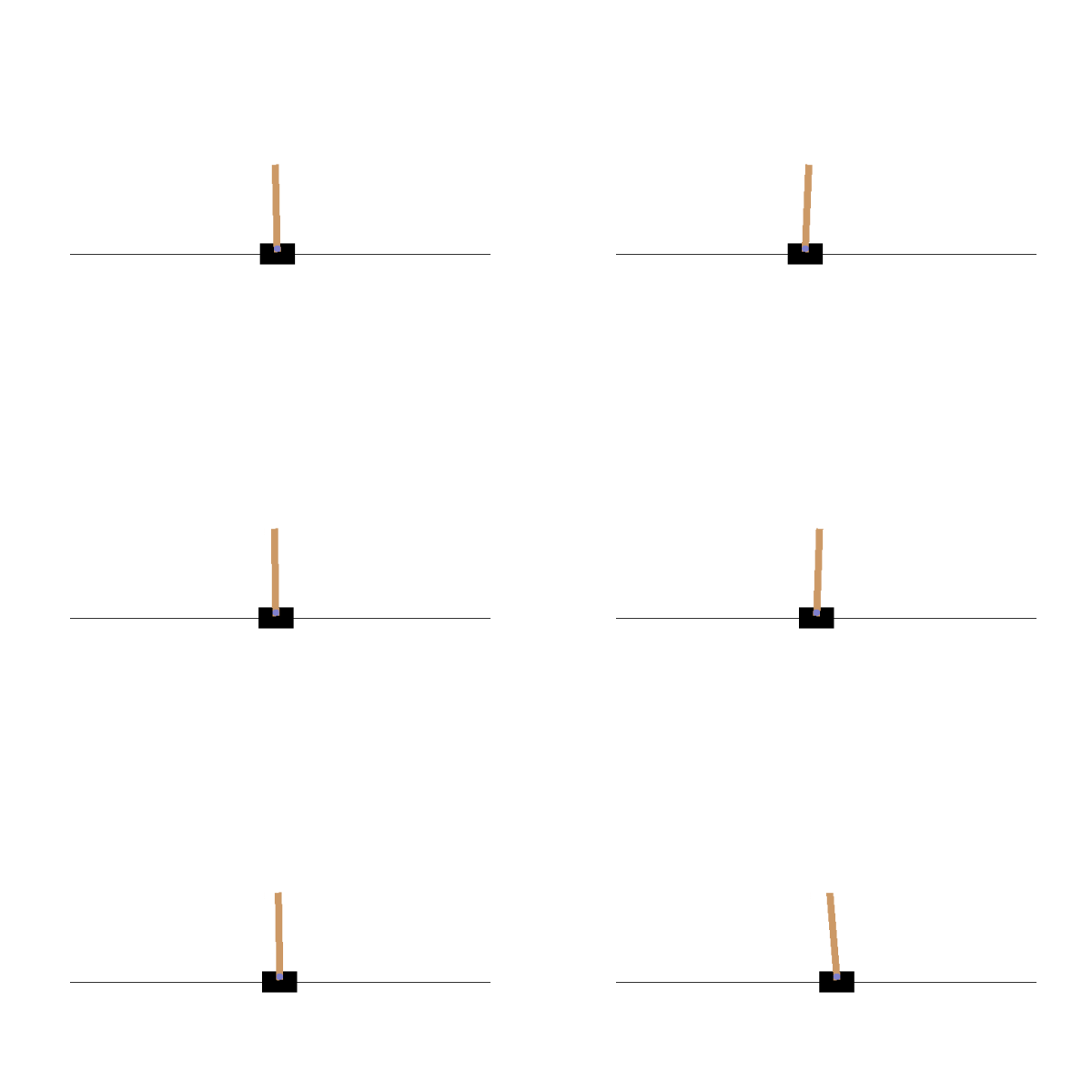
To demonstrate BC we’ve chosen a simple graphical environment in the Open AI gym, called cartpole\. The agent consists of a cart set on a frictionless surface with a frictionless joint that attaches a pole on top\. The goal of the agent is to balance this pole\. It has a discrete action space: \{push to the left \- 0, push to the right \- 1\} and a continuous state space: \{cart position \- \[\-4\.8, 4\.8\] , cart velocity \- \[\-inf, inf\] , pole angle \- \[\-24, 24 \(deg\)\], pole angular velocity \- \[\-inf, inf\]\}\.
To obtain expert demostrations, we quickly train Open AI’s PPO implementation and sample from it’s trained agent\. Now, we are left with the supervised learning problem which is the crux of BC\. We go about solving this supervised learning problem using a fully connected neural net with three layers follow by ReLU nonlinearities and a final sigmoid nonlinearity\. Given the training data, we can now approximate a function that maps states to actions, which serves as your behaviorally cloned policy\.
Although our expert PPO agent is familiar with the reward structure of the environment, we can achieve similar performance without knowing the underlying MDP\. But, when our trained agent interacts with states not covered by the expert demostrator, it won’t know how to behave\. This issue, refered to as distribution shift, can cause a compounding sequence of incorrect steps that wreck havoc\. If a BC agent encounters a state that it is even slightly unfamiliar, it will take a wrong action, leading it towards a next state even more unfamiliar — diverging from the expert very easily\. When it came to our specific task, we tried our best to engineer around this issue and others that arose — see below\.
During the process of training the behavioral cloning net, a few engineering tricks were required to get the clone working, listed below for reference\.
\(1\) Adding a final sigmoid \(i\.e\. not TanH or ReLU\) nonlinearity to account for the binary actions and to avoid numerical instability \(2\) Generating more sample data from the expert if too few isn’t sufficient enough to cover the intricate expert behavior \(3\) Not making the model too deep to prevent overfitting \(4\) Performing a hyperparameter search on the learning rate
These steps above allowed the BC agent to transform from a cart that couldn’t even hold the pole up to one that can now balance it for multiple steps\. In early experiments, I didn’t sample enough expert points to really learn the non\-linear dynamics of the expert cartpole, so I needed to make sure to generate sufficient sample data\. I also noticed my initial net was outputing actions that were integers outside the action space \(i\.e\. \-1 or 3\), so I had to add the sigmoid to rescrict this behavior and improve numerical stabilty\. Finally, I had to tune the model depth and learning rate to handle jittery behavior that was likely due to overfitting and convergence to local optimums, respectively\. There are many more engineering methods I could continue pursuing to ensure better performance, but I stopped once I was able to demonstrate successful learned behavior with the clone\.
```
'''
Imports
'''
import numpy as np
import torch
import torch.nn as nn
import torch.nn.functional as F
import gym
from stable_baselines.common.policies import MlpPolicy
from stable_baselines import PPO1
from stable_baselines.gail import generate_expert_traj
'''
Create Env and Train Expert
'''
env = gym.make('CartPole-v1')
model = PPO1(MlpPolicy, env, verbose=1)
model.learn(total_timesteps=250000)
model.save("ppo1_cartpole")
model = PPO1.load("ppo1_cartpole")
'''
Generate Expert Demonstrations
Specs:
No. of Trajectories: 1000
No. of State action Pairs: 479318
Model: PPO (taken from Open AI Baseline Implementation)
'''
size = 1000
generate_expert_traj(model, 'expert_cartpole', env = env , n_timesteps=0, n_episodes=size)
demos = np.load('expert_cartpole.npz', mmap_mode='r')
data_in = demos['obs']
data_out = demos['actions']
'''
Define BC Model as NN
Specs:
NN: 3 layers (4 each cells with ReLu) and Sigmoid on Output
Loss: BCE (Binary Cross Entropy)
'''
class Net(nn.Module):
def __init__(self):
super(Net, self).__init__()
self.fc1 = nn.Linear(4, 4)
self.fc2 = nn.Linear(4, 4)
self.fc3 = nn.Linear(4, 1)
def forward(self, x):
x = F.relu(self.fc1(x))
x = F.relu(self.fc2(x))
x = F.sigmoid(self.fc3(x))
return x
net = Net()
model = net
'''
Train BC Model
'''
criterion = nn.BCELoss()
learning_rate = [10, 1, 0.1, 0.01, 0.001, 0.0001]
#learning_rate that worke = [1.5]
for lr in learning_rate:
x = torch.from_numpy(data_in).to(torch.float32)
y = torch.from_numpy(data_out).to(torch.float32)
for t in range(200):
y_pred = model(x)
loss = criterion(y_pred, y)
print(t, loss.item())
model.zero_grad()
loss.backward()
with torch.no_grad():
for param in model.parameters():
param.data -= lr * param.grad
'''
Render BC Agent and Generate Gifs
'''
env = gym.make('CartPole-v1')
obs = env.reset()
#frames = []
T = 200
for t in range(T):
obs = torch.from_numpy(obs)
model.double()
action = model.forward(obs)
if action < 0.5:
action = 0
else:
action = 1
#print(action)
obs, rewards, dones, info = env.step(action)
#print(obs)
env.render()
time.sleep(.025)
#frames.append(env.render(mode="rgb_array"))
```
[](https://substackcdn.com/image/fetch/$s_!oiq-!,f_auto,q_auto:good,fl_progressive:steep/https%3A%2F%2Fsubstack-post-media.s3.amazonaws.com%2Fpublic%2Fimages%2F50cf649d-afc1-498e-a279-2baf089a8596_600x400.gif)
[](https://substackcdn.com/image/fetch/$s_!HqKj!,f_auto,q_auto:good,fl_progressive:steep/https%3A%2F%2Fsubstack-post-media.s3.amazonaws.com%2Fpublic%2Fimages%2F84b312f2-7150-464e-aec6-f8488ebc47df_600x400.gif)
As you can see, it doesn’t do terribly well, it’s merely a budget PPO\. However, with more model engineering, and cherry picked initialization data, you could see better results\.
If this material interests you, read more about Behavioral Cloning and other Imitation Learning methods in the references below\. In addition, I would like to acknowledge a few people for their key contributions: \(1\) Charlie Snell for helping debug the BC Net and imparting his engineering experience with the gym and training agents \(2\) Aurick Zhou for explaining the intuition behind BC and it’s connection with MLE\.
- Survey paper on Imitation Learning\.[https://arxiv\.org/pdf/1811\.06711\.pdf](https://arxiv.org/pdf/1811.06711.pdf)
- Introduction to Probability by Bertsekas and Tsitsiklis\. Example 3\.11 on Buffon’s Needle and Chapt 9\.1 on Classical Parameter Estimation
- Wiki on Likelihood\.[https://en\.wikipedia\.org/wiki/Likelihood\_function](https://en.wikipedia.org/wiki/Likelihood_function)
- BC Self\-driving paper \(ALVINN\)\.[https://papers\.nips\.cc/paper/1988/file/812b4ba287f5ee0bc9d43bbf5bbe87fb\-Paper\.pdf](https://papers.nips.cc/paper/1988/file/812b4ba287f5ee0bc9d43bbf5bbe87fb-Paper.pdf)
- First Alpha\-go paper\.[https://www\.nature\.com/articles/nature16961](https://www.nature.com/articles/nature16961)
- Imitation Learning github reopo\.[https://github\.com/HumanCompatibleAI/imitation](https://github.com/HumanCompatibleAI/imitation)
- PPO model documentation\.[https://stable\-baselines\.readthedocs\.io/en/master/modules/ppo2\.html](https://stable-baselines.readthedocs.io/en/master/modules/ppo2.html)
- Dataset collection documentation\.[https://stable\-baselines\.readthedocs\.io/en/master/guide/pretrain\.html](https://stable-baselines.readthedocs.io/en/master/guide/pretrain.html)
- Cartpole Tutorial\.[https://xaviergeerinck\.com/post/ai/rl/openai\-cartpole](https://xaviergeerinck.com/post/ai/rl/openai-cartpole)
- OpenAI Gym Cartpole env\.[https://github\.com/openai/gym/blob/master/gym/envs/classic\_control/cartpole\.py](https://github.com/openai/gym/blob/master/gym/envs/classic_control/cartpole.py)
- Pytorch RL tutorial\.[https://pytorch\.org/tutorials/intermediate/reinforcement\_q\_learning\.html](https://pytorch.org/tutorials/intermediate/reinforcement_q_learning.html)
- Pytorch basics tutorial\.[https://pytorch\.org/tutorials/beginner/blitz/cifar10\_tutorial\.html](https://pytorch.org/tutorials/beginner/blitz/cifar10_tutorial.html)
- Another pytorch basics tutorial\.[https://github\.com/jcjohnson/pytorch\-examples](https://github.com/jcjohnson/pytorch-examples)
- Yet another pytorch basics tutorial\.[https://pytorch\.org/tutorials/beginner/blitz/neural\_networks\_tutorial\.html](https://pytorch.org/tutorials/beginner/blitz/neural_networks_tutorial.html)
- Gym gif renderer\.[https://gist\.github\.com/botforge/64cbb71780e6208172bbf03cd9293553](https://gist.github.com/botforge/64cbb71780e6208172bbf03cd9293553)
#### Discussion about this post
### Ready for more?
BCL is the first optimization framework that uses particle filtering with Bayesian updates to systematically refine label representations for information extraction tasks, showing consistent improvements over existing methods.
BPCO introduces a stable recipe for critic-based reinforcement learning in language models, combining bounded value predictions and Monte Carlo targets to match group-based methods with single-response sampling.
CBPO introduces a contrastive branch policy optimization method for fine-grained credit assignment in reinforcement learning with verifiable rewards, enhancing language model performance in tool-integrated reasoning tasks across multiple benchmarks.
BiPACE introduces a drop-in advantage estimator that fixes state-action credit mismatch in stepwise group-based RL for LLM agents, using bisimulation-guided state clustering and action counterfactual estimation, achieving significant performance gains on ALFWorld, WebShop, and TextCraft with Qwen2.5 models.
The paper proposes BC-ICL, a bootstrap-conditioned action selection method that leverages pretrained tabular foundation models with in-context learning for contextual bandits, improving exploration and regret performance under strict online protocols.