Imitation Learning: How well does it perform?

ML at Berkeley 04/28/21, 12:30 PM Papers

Summary

This article analyzes a recent research paper that provides a taxonomical framework for imitation learning algorithms, categorizing them by moment matching techniques and analyzing their theoretical imitation gap bounds.

<p><em>By Surya Vengadesan</em></p><p>Imitation learning (IL) broadly encompasses any algorithm (e.g. <a href="https://ml.berkeley.edu/blog/posts/bc/">BC</a>) that attempts to learn a policy for an <a href="https://ml.berkeley.edu/blog/posts/mdps/">MDP</a> given expert demonstrations. In this blog post, we will be discussing how one can distinguish this task into three subclasses of IL algorithms with some mathematical rigor. In particular, we will be describing ideas presented in this recent <a href="https://arxiv.org/abs/2103.03236">paper</a> that provides a taxonomixal framework for imitation learning algorithms.</p><p>A key idea behind this paper is to define a metric that generalizes the goal of IL algorithms at large. Simply put, find a policy that minimizes the <em>imitation gap</em> <em>J(π<sub>E</sub>)−J(π)</em>, between our learned policy <em>π</em> and an expert policy <em>π<sub>E</sub></em>. In particular, we define <em>J(⋅)</em>, what we call a moment, which is the expection over some function.</p><p>The goal is to then match the expert and learner moments, which the paper refers to as moment matching. In particular each type of IL algorithm can be defined by different types of moments being matched, such as reward or Q functions. Through this lens, IL can be viewed as applying optimization techniques to minimize the imitation gap.</p><p>The paper then goes onto clearly defining the three types of IL algorithms and provides each with theoretical guarantees, proof after proof. Specifically, the author delineates between (1) matching rewards with access to the environment (2) matching q-values with access to the environment (3) matching q-values without access to the environment.</p><p>Now, we’ll attempt to deconstruct proofs from the paper on whether an algorithm’s imitation gap grows linearly or quadratically in time.</p><div class="captioned-image-container"><figure><a class="image-link image2 is-viewable-img" target="_blank" href="https://substackcdn.com/image/fetch/$s_!eOZL!,f_auto,q_auto:good,fl_progressive:steep/https%3A%2F%2Fsubstack-post-media.s3.amazonaws.com%2Fpublic%2Fimages%2Fcf245843-c3c2-4d51-b6ec-2736bd14c790_1200x630.jpeg" data-component-name="Image2ToDOM"><div class="image2-inset"><picture><source type="image/webp" srcset="https://substackcdn.com/image/fetch/$s_!eOZL!,w_424,c_limit,f_webp,q_auto:good,fl_progressive:steep/https%3A%2F%2Fsubstack-post-media.s3.amazonaws.com%2Fpublic%2Fimages%2Fcf245843-c3c2-4d51-b6ec-2736bd14c790_1200x630.jpeg 424w, https://substackcdn.com/image/fetch/$s_!eOZL!,w_848,c_limit,f_webp,q_auto:good,fl_progressive:steep/https%3A%2F%2Fsubstack-post-media.s3.amazonaws.com%2Fpublic%2Fimages%2Fcf245843-c3c2-4d51-b6ec-2736bd14c790_1200x630.jpeg 848w, https://substackcdn.com/image/fetch/$s_!eOZL!,w_1272,c_limit,f_webp,q_auto:good,fl_progressive:steep/https%3A%2F%2Fsubstack-post-media.s3.amazonaws.com%2Fpublic%2Fimages%2Fcf245843-c3c2-4d51-b6ec-2736bd14c790_1200x630.jpeg 1272w, https://substackcdn.com/image/fetch/$s_!eOZL!,w_1456,c_limit,f_webp,q_auto:good,fl_progressive:steep/https%3A%2F%2Fsubstack-post-media.s3.amazonaws.com%2Fpublic%2Fimages%2Fcf245843-c3c2-4d51-b6ec-2736bd14c790_1200x630.jpeg 1456w" sizes="100vw"><img src="https://substackcdn.com/image/fetch/$s_!eOZL!,w_1456,c_limit,f_auto,q_auto:good,fl_progressive:steep/https%3A%2F%2Fsubstack-post-media.s3.amazonaws.com%2Fpublic%2Fimages%2Fcf245843-c3c2-4d51-b6ec-2736bd14c790_1200x630.jpeg" width="1200" height="630" data-attrs="{"src":"https://substack-post-media.s3.amazonaws.com/public/images/cf245843-c3c2-4d51-b6ec-2736bd14c790_1200x630.jpeg","srcNoWatermark":null,"fullscreen":null,"imageSize":null,"height":630,"width":1200,"resizeWidth":null,"bytes":null,"alt":null,"title":null,"type":null,"href":null,"belowTheFold":false,"topImage":true,"internalRedirect":null,"isProcessing":false,"align":null,"offset":false}" class="sizing-normal" alt="" srcset="https://substackcdn.com/image/fetch/$s_!eOZL!,w_424,c_limit,f_auto,q_auto:good,fl_progressive:steep/https%3A%2F%2Fsubstack-post-media.s3.amazonaws.com%2Fpublic%2Fimages%2Fcf245843-c3c2-4d51-b6ec-2736bd14c790_1200x630.jpeg 424w, https://substackcdn.com/image/fetch/$s_!eOZL!,w_848,c_limit,f_auto,q_auto:good,fl_progressive:steep/https%3A%2F%2Fsubstack-post-media.s3.amazonaws.com%2Fpublic%2Fimages%2Fcf245843-c3c2-4d51-b6ec-2736bd14c790_1200x630.jpeg 848w, https://substackcdn.com/image/fetch/$s_!eOZL!,w_1272,c_limit,f_auto,q_auto:good,fl_progressive:steep/https%3A%2F%2Fsubstack-post-media.s3.amazonaws.com%2Fpublic%2Fimages%2Fcf245843-c3c2-4d51-b6ec-2736bd14c790_1200x630.jpeg 1272w, https://substackcdn.com/image/fetch/$s_!eOZL!,w_1456,c_limit,f_auto,q_auto:good,fl_progressive:steep/https%3A%2F%2Fsubstack-post-media.s3.amazonaws.com%2Fpublic%2Fimages%2Fcf245843-c3c2-4d51-b6ec-2736bd14c790_1200x630.jpeg 1456w" sizes="100vw" fetchpriority="high"></picture><div class="image-link-expand"><div class="pencraft pc-display-flex pc-gap-8 pc-reset"><button tabindex="0" type="button" class="pencraft pc-reset pencraft icon-container restack-image"><svg role="img" width="20" height="20" viewBox="0 0 20 20" fill="none" stroke-width="1.5" stroke="var(--color-fg-primary)" stroke-linecap="round" stroke-linejoin="round" xmlns="http://www.w3.org/2000/svg"><g><title></title><path d="M2.53001 7.81595C3.49179 4.73911 6.43281 2.5 9.91173 2.5C13.1684 2.5 15.9537 4.46214 17.0852 7.23684L17.6179 8.67647M17.6179 8.67647L18.5002 4.26471M17.6179 8.67647L13.6473 6.91176M17.4995 12.1841C16.5378 15.2609 13.5967 17.5 10.1178 17.5C6.86118 17.5 4.07589 15.5379 2.94432 12.7632L2.41165 11.3235M2.41165 11.3235L1.5293 15.7353M2.41165 11.3235L6.38224 13.0882"></path></g></svg></button><button tabindex="0" type="button" class="pencraft pc-reset pencraft icon-container view-image"><svg xmlns="http://www.w3.org/2000/svg" width="20" height="20" viewBox="0 0 24 24" fill="none" stroke="currentColor" stroke-width="2" stroke-linecap="round" stroke-linejoin="round" class="lucide lucide-maximize2 lucide-maximize-2"><polyline points="15 3 21 3 21 9"></polyline><polyline points="9 21 3 21 3 15"></polyline><line x1="21" x2="14" y1="3" y2="10"></line><line x1="3" x2="10" y1="21" y2="14"></line></svg></button></div></div></div></a></figure></div><p>In particular, we will cover the paper’s first lemma which proves a linear upper bound on the imitation gap for type (1) algorithms that moment match reward functions like <a href="https://arxiv.org/abs/1606.03476">GAIL</a> or <a href="https://arxiv.org/abs/1905.11108">SQIL</a>. In the process, we will breakdown this craft of proving algorithmic bounds, then welcome the reader to decode the remaining proofs.</p><p><em>Lemma 1</em>: Reward Upper Bound: If <em>F<sub>r</sub></em> spans F, then for all MDPs, <em>π<sub>E</sub></em> and π←Ψ{ϵ}</p><div class="latex-rendered" data-attrs="{"persistentExpression":"J(\\pi_E) - J(\\pi) \\leq O(\\epsilon T)","id":"AISAHEBFYD"}" data-component-name="LatexBlockToDOM"></div><p>That sounds like a handful; now, let’s break this down.</p><p>The author precedes this lemma with general framework that formalizes the goal of imitation learning algorithms. We should look at imitation learning as a two-player game. We define the payoff function of this game with <em>U<sub>1</sub></em> as follows:</p><div class="latex-rendered" data-attrs="{"persistentExpression":"U_1(\\pi, f) = \\frac{1}{T}(\\mathbb{E}_{\\tau \\sim \\pi}[\\Sigma_{t=1}^{T} f(s_t, a_t)] - \\mathbb{E}_{\\tau \\sim \\pi_E}[\\Sigma_{t=1}^{T} f(s_t, a_t)])","id":"AFBIRERVOE"}" data-component-name="LatexBlockToDOM"></div><p>Above, see the difference between two moments, the first moment over the sum of rewards till a time horizon T while following policy <em>π</em>, and the second moment over the sum of rewards till the same time horizon but following the expert policy <em>π<sub>E</sub></em>. Therefore, given some expert policy <em>π<sub>E</sub></em>, the game is to choose a policy <em>π</em> that best matches the moment of the expert, while being robust to all possible MDP reward functions <em>f</em>.</p><p>The paper defines Player 1 as the IL algorithm that attempts to select some policy <em>π</em> from the set of all possible policies </p><div class="latex-rendered" data-attrs="{"persistentExpression":"\\Pi = \\ \\{\\pi: \\mathcal{S} \\to \\Delta(\\mathcal{A})\\}","id":"YSHOVBLGMO"}" data-component-name="LatexBlockToDOM"></div><p>and whose goal is to minimize the imitation gap <em>U<sub>1</sub></em>. Player 2 is a discriminating reward function <em>f</em> selected from the set of all reward functions F<sub>r</sub>={S x A→[−1,1]}, whose goal is to maximize the imitation gap <em>U<sub>1</sub></em>.</p><p>The notion of an δ-approximate solution to this game is also introduced. Given a payoff <em>U<sub>j</sub></em>, a pair (f^,π^) is a δ-eq. solution if:</p><div class="latex-rendered" data-attrs="{"persistentExpression":"sup_{f \\in \\mathcal{F}}U_j(f, \\hat{\\pi}) - \\frac{\\delta}{2} \\leq U_j(\\hat{f}, \\hat{\\pi}) \\leq inf_{\\pi \\in \\Pi} U_j(\\hat{f}, \\pi) + \\frac{\\delta}{2}","id":"OVXWLMQUPZ"}" data-component-name="LatexBlockToDOM"></div><p>In addition, we define a function that magically solves this game for us, which we call the imitation game δ-oracle, Ψ{δ}(⋅), which takes in in a payoff function </p><div class="latex-rendered" data-attrs="{"persistentExpression":"U: \\Pi \\times \\mathcal{F} \\to [-k, k]","id":"PQTXJFKISK"}" data-component-name="LatexBlockToDOM"></div><p>and returns a (<em>k</em>δ)-approximate equilibrium solution (f^,π^) that satifies the condition above.</p><p>Using the tools built up, we can now prove lemma 1. First one needs to use the imitation gap, based on it’s definition in the paper:</p><div class="latex-rendered" data-attrs="{"persistentExpression":"J(\\pi_E) - J(\\pi) \\leq sup_{f \\in \\mathcal{F}_r} \\mathbb{E}_{\\tau \\sim \\pi}\\Sigma_{t = 1}^{T} f(s_t, a_t) - \\mathbb{E}_{\\tau \\sim \\pi_E}\\Sigma_{t=1}^{T}f(s_t, a_t)","id":"DMSPIJNJAC"}" data-component-name="LatexBlockToDOM"></div><p>Next, since the sup is always positive, we can multiply by it by two and the new sup will be greater than one above. In addition, by defintion of <em>U<sub>1</sub></em>, you can see that term we are taking the supremum over is simply <em>T</em> multiplied by <em>U<sub>1</sub></em>. Therefore, we have: </p><div class="latex-rendered" data-attrs="{"persistentExpression":"J(\\pi_E) - J(\\pi) \\leq 2T sup_{f \\in \\mathcal{F}} U_1(\\pi, f)","id":"KUDKHPIKVP"}" data-component-name="LatexBlockToDOM"></div><p>Finally, if we apply the δ-approx. equilibrium def, we can see that: </p><div class="latex-rendered" data-attrs="{"persistentExpression":"sup_{f \\in \\mathcal{F}} U_j(f, \\hat{\\pi}) - \\frac{\\delta}{2} \\leq U_j(\\hat{f}, \\hat{\\pi})","id":"WYGREPUYZI"}" data-component-name="LatexBlockToDOM"></div><p>Where f^ and π^, the optimal values can be seen as the result of performing the minimax over the policy class Π:</p><div class="latex-rendered" data-attrs="{"persistentExpression":"min_{\\pi \\in \\Pi} max_{f \\in \\mathcal{F}}U_j(\\pi, f)","id":"ANVYKMPQKV"}" data-component-name="LatexBlockToDOM"></div><p>which is equal to 0 since, the expert policy <em>π<sub>E</sub></em>∈Π, so <em>U<sub>1</sub></em> (as further defined above) collapses to 0.</p><p>Finally, we have that </p><div class="latex-rendered" data-attrs="{"persistentExpression":"sup_{f \\in \\mathcal{F}} U_1(f, \\hat{\\pi})- \\frac{\\delta}{2} \\leq 0","id":"CUDIXGSNKI"}" data-component-name="LatexBlockToDOM"></div><p>and if you multiply this inequality by <em>2T</em>, and bring the δ term to the right, you get </p><div class="latex-rendered" data-attrs="{"persistentExpression":"2T sup_{f \\in \\mathcal{F}}U_1(\\pi, f) \\leq 2T\\delta","id":"JIFEPIDISW"}" data-component-name="LatexBlockToDOM"></div><p>This matches the ϵ definition from the Lemma 1, so we finally get </p><div class="latex-rendered" data-attrs="{"persistentExpression":"J(\\pi_{E}) - L(\\pi) \\leq 2T\\epsilon = O(\\epsilon T)","id":"TDQOSXJKZL"}" data-component-name="LatexBlockToDOM"></div><p>The other lemma then goes onto proving that the lowerboard is also linearly constrainted.</p><p><em>Lemma 2</em>: There exists an MDP, <em>π<sub>E</sub></em>, and <em>π←Ψ{ϵ}(U<sub>1</sub>)</em> such that </p><div class="latex-rendered" data-attrs="{"persistentExpression":"J(\\pi_E) - J(\\pi) \\geq \\Omega(\\epsilon T)","id":"BYRKVYMCBT"}" data-component-name="LatexBlockToDOM"></div><p>However, takes on different techniques to prove the statement, which requires an in-depth understanding of more definitions to creatively chain together multiple logical tricks. Together, lemma 1 and 2 show that for any IL algorithm that attempts to match reward moments, its imitation gap will grow linear in both the best and worst case scenarios.</p><p>The paper goes on to prove bounds for the other two taxonomical categories, introduces a mathematical concept on MDPs called “recoverability”, and proposes two new algorithms using the proven bounds, one of which is called Adversarial Reward-moment Imitation Learning that is claimed to perform with better guaranteed performance over SQIL and GAIL.</p><p>If this material sounds interesting, check out the further readings below to get a glimpse into the world of Imitation Learning and how researchers today are incorporating rigor into the field in creative ways.</p><p>Also check out this <a href="https://www.youtube.com/playlist?list=PL51kEpt5uSsbZSaGyUMsLsOoFP8-hyx0R">youtube playlist</a> created by Swamy et al. which gives an excellent overview of the work discussed in this blog.</p><h2>References</h2><ul><li><p><a href="https://www.youtube.com/playlist?list=PL51kEpt5uSsbZSaGyUMsLsOoFP8-hyx0R">https://www.youtube.com/playlist?list=PL51kEpt5uSsbZSaGyUMsLsOoFP8-hyx0R</a></p></li><li><p><a href="https://arxiv.org/pdf/2009.05990.pdf">https://arxiv.org/pdf/2009.05990.pdf</a></p></li><li><p><a href="http://proceedings.mlr.press/v9/ross10a.html">http://proceedings.mlr.press/v9/ross10a.html</a></p></li><li><p><a href="http://proceedings.mlr.press/v9/ross10a/ross10aSupple.pdf">http://proceedings.mlr.press/v9/ross10a/ross10aSupple.pdf</a></p></li><li><p><a href="https://inst.eecs.berkeley.edu/~cs188/sp21/assets/notes/note02.pdf">https://inst.eecs.berkeley.edu/~cs188/sp21/assets/notes/note02.pdf</a></p></li><li><p><a href="https://www.youtube.com/watch?v=XqgDtD_P75A&feature=emb_logo">https://www.youtube.com/watch?v=XqgDtD_P75A&feature=emb_logo</a></p></li></ul>

Original Article

View Cached Full Text

Cached at: 05/08/26, 08:42 AM

# Imitation Learning: How well does it perform? Source: [https://mlberkeley.substack.com/p/il](https://mlberkeley.substack.com/p/il) *By Surya Vengadesan* Imitation learning $IL$ broadly encompasses any algorithm $e\.g\.[BC](https://ml.berkeley.edu/blog/posts/bc/)$ that attempts to learn a policy for an[MDP](https://ml.berkeley.edu/blog/posts/mdps/)given expert demonstrations\. In this blog post, we will be discussing how one can distinguish this task into three subclasses of IL algorithms with some mathematical rigor\. In particular, we will be describing ideas presented in this recent[paper](https://arxiv.org/abs/2103.03236)that provides a taxonomixal framework for imitation learning algorithms\. A key idea behind this paper is to define a metric that generalizes the goal of IL algorithms at large\. Simply put, find a policy that minimizes the*imitation gap**J$πE$−J$π$*, between our learned policy*π*and an expert policy*πE*\. In particular, we define*J$⋅$*, what we call a moment, which is the expection over some function\. The goal is to then match the expert and learner moments, which the paper refers to as moment matching\. In particular each type of IL algorithm can be defined by different types of moments being matched, such as reward or Q functions\. Through this lens, IL can be viewed as applying optimization techniques to minimize the imitation gap\. The paper then goes onto clearly defining the three types of IL algorithms and provides each with theoretical guarantees, proof after proof\. Specifically, the author delineates between $1$ matching rewards with access to the environment $2$ matching q\-values with access to the environment $3$ matching q\-values without access to the environment\. Now, we’ll attempt to deconstruct proofs from the paper on whether an algorithm’s imitation gap grows linearly or quadratically in time\. 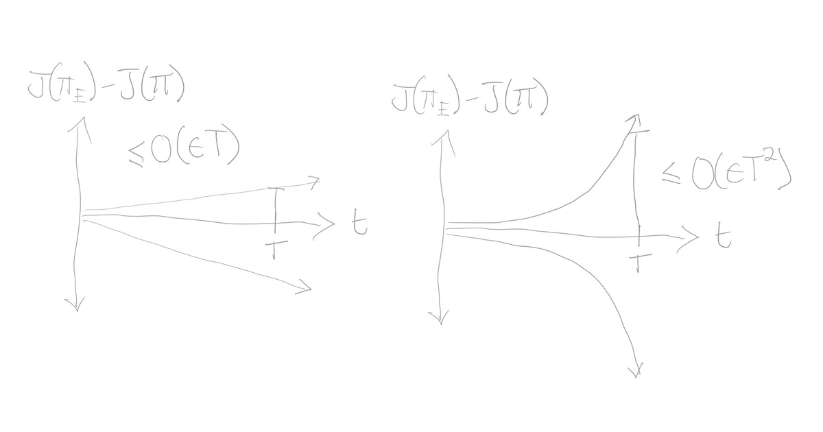[![](https://substackcdn.com/image/fetch/$s_!eOZL!,w_1456,c_limit,f_auto,q_auto:good,fl_progressive:steep/https%3A%2F%2Fsubstack-post-media.s3.amazonaws.com%2Fpublic%2Fimages%2Fcf245843-c3c2-4d51-b6ec-2736bd14c790_1200x630.jpeg)](https://substackcdn.com/image/fetch/$s_!eOZL!,f_auto,q_auto:good,fl_progressive:steep/https%3A%2F%2Fsubstack-post-media.s3.amazonaws.com%2Fpublic%2Fimages%2Fcf245843-c3c2-4d51-b6ec-2736bd14c790_1200x630.jpeg) In particular, we will cover the paper’s first lemma which proves a linear upper bound on the imitation gap for type $1$ algorithms that moment match reward functions like[GAIL](https://arxiv.org/abs/1606.03476)or[SQIL](https://arxiv.org/abs/1905.11108)\. In the process, we will breakdown this craft of proving algorithmic bounds, then welcome the reader to decode the remaining proofs\. *Lemma 1*: Reward Upper Bound: If*Fr*spans F, then for all MDPs,*πE* and π←Ψ\{ϵ\} \\$J\(\\pi\_E$ \- J$\\pi$ \\leq O$\\epsilon T$\\\) That sounds like a handful; now, let’s break this down\. The author precedes this lemma with general framework that formalizes the goal of imitation learning algorithms\. We should look at imitation learning as a two\-player game\. We define the payoff function of this game with*U1*as follows: \\$U\_1\(\\pi, f$ = \\frac\{1\}\{T\}$\\mathbb\{E\}\_\{\\tau \\sim \\pi\}\[\\Sigma\_\{t=1\}^\{T\} f\(s\_t, a\_t$\] \- \\mathbb\{E\}\_\{\\tau \\sim \\pi\_E\}\[\\Sigma\_\{t=1\}^\{T\} f$s\_t, a\_t$\]\)\\\) Above, see the difference between two moments, the first moment over the sum of rewards till a time horizon T while following policy*π*, and the second moment over the sum of rewards till the same time horizon but following the expert policy*πE*\. Therefore, given some expert policy*πE*, the game is to choose a policy*π*that best matches the moment of the expert, while being robust to all possible MDP reward functions*f*\. The paper defines Player 1 as the IL algorithm that attempts to select some policy*π*from the set of all possible policies \\$\\Pi = \\ \\\{\\pi: \\mathcal\{S\} \\to \\Delta\(\\mathcal\{A\}$\\\}\\\) and whose goal is to minimize the imitation gap*U1*\. Player 2 is a discriminating reward function*f*selected from the set of all reward functions Fr=\{S x A→\[−1,1\]\}, whose goal is to maximize the imitation gap*U1*\. The notion of an δ\-approximate solution to this game is also introduced\. Given a payoff*Uj*, a pair $f^,π^$ is a δ\-eq\. solution if: \\$sup\_\{f \\in \\mathcal\{F\}\}U\_j\(f, \\hat\{\\pi\}$ \- \\frac\{\\delta\}\{2\} \\leq U\_j$\\hat\{f\}, \\hat\{\\pi\}$ \\leq inf\_\{\\pi \\in \\Pi\} U\_j$\\hat\{f\}, \\pi$ \+ \\frac\{\\delta\}\{2\}\\\) In addition, we define a function that magically solves this game for us, which we call the imitation game δ\-oracle, Ψ\{δ\}$⋅$, which takes in in a payoff function \\$U: \\Pi \\times \\mathcal\{F\} \\to \[\-k, k\]\\$ and returns a $*k*δ$\-approximate equilibrium solution $f^,π^$ that satifies the condition above\. Using the tools built up, we can now prove lemma 1\. First one needs to use the imitation gap, based on it’s definition in the paper: \\$J\(\\pi\_E$ \- J$\\pi$ \\leq sup\_\{f \\in \\mathcal\{F\}\_r\} \\mathbb\{E\}\_\{\\tau \\sim \\pi\}\\Sigma\_\{t = 1\}^\{T\} f$s\_t, a\_t$ \- \\mathbb\{E\}\_\{\\tau \\sim \\pi\_E\}\\Sigma\_\{t=1\}^\{T\}f$s\_t, a\_t$\\\) Next, since the sup is always positive, we can multiply by it by two and the new sup will be greater than one above\. In addition, by defintion of*U1*, you can see that term we are taking the supremum over is simply*T*multiplied by*U1*\. Therefore, we have: \\$J\(\\pi\_E$ \- J$\\pi$ \\leq 2T sup\_\{f \\in \\mathcal\{F\}\} U\_1$\\pi, f$\\\) Finally, if we apply the δ\-approx\. equilibrium def, we can see that: \\$sup\_\{f \\in \\mathcal\{F\}\} U\_j\(f, \\hat\{\\pi\}$ \- \\frac\{\\delta\}\{2\} \\leq U\_j$\\hat\{f\}, \\hat\{\\pi\}$\\\) Where f^ and π^, the optimal values can be seen as the result of performing the minimax over the policy class Π: \\$min\_\{\\pi \\in \\Pi\} max\_\{f \\in \\mathcal\{F\}\}U\_j\(\\pi, f$\\\) which is equal to 0 since, the expert policy*πE*∈Π, so*U1* $as further defined above$ collapses to 0\. Finally, we have that \\$sup\_\{f \\in \\mathcal\{F\}\} U\_1\(f, \\hat\{\\pi\}$\- \\frac\{\\delta\}\{2\} \\leq 0\\\) and if you multiply this inequality by*2T*, and bring the δ term to the right, you get \\$2T sup\_\{f \\in \\mathcal\{F\}\}U\_1\(\\pi, f$ \\leq 2T\\delta\\\) This matches the ϵ definition from the Lemma 1, so we finally get \\$J\(\\pi\_\{E\}$ \- L$\\pi$ \\leq 2T\\epsilon = O$\\epsilon T$\\\) The other lemma then goes onto proving that the lowerboard is also linearly constrainted\. *Lemma 2*: There exists an MDP,*πE*, and*π←Ψ\{ϵ\}$U1$*such that \\$J\(\\pi\_E$ \- J$\\pi$ \\geq \\Omega$\\epsilon T$\\\) However, takes on different techniques to prove the statement, which requires an in\-depth understanding of more definitions to creatively chain together multiple logical tricks\. Together, lemma 1 and 2 show that for any IL algorithm that attempts to match reward moments, its imitation gap will grow linear in both the best and worst case scenarios\. The paper goes on to prove bounds for the other two taxonomical categories, introduces a mathematical concept on MDPs called “recoverability”, and proposes two new algorithms using the proven bounds, one of which is called Adversarial Reward\-moment Imitation Learning that is claimed to perform with better guaranteed performance over SQIL and GAIL\. If this material sounds interesting, check out the further readings below to get a glimpse into the world of Imitation Learning and how researchers today are incorporating rigor into the field in creative ways\. Also check out this[youtube playlist](https://www.youtube.com/playlist?list=PL51kEpt5uSsbZSaGyUMsLsOoFP8-hyx0R)created by Swamy et al\. which gives an excellent overview of the work discussed in this blog\. - [https://www\.youtube\.com/playlist?list=PL51kEpt5uSsbZSaGyUMsLsOoFP8\-hyx0R](https://www.youtube.com/playlist?list=PL51kEpt5uSsbZSaGyUMsLsOoFP8-hyx0R) - [https://arxiv\.org/pdf/2009\.05990\.pdf](https://arxiv.org/pdf/2009.05990.pdf) - [http://proceedings\.mlr\.press/v9/ross10a\.html](http://proceedings.mlr.press/v9/ross10a.html) - [http://proceedings\.mlr\.press/v9/ross10a/ross10aSupple\.pdf](http://proceedings.mlr.press/v9/ross10a/ross10aSupple.pdf) - [https://inst\.eecs\.berkeley\.edu/~cs188/sp21/assets/notes/note02\.pdf](https://inst.eecs.berkeley.edu/~cs188/sp21/assets/notes/note02.pdf) - [https://www\.youtube\.com/watch?v=XqgDtD\_P75A&feature=emb\_logo](https://www.youtube.com/watch?v=XqgDtD_P75A&feature=emb_logo) #### Discussion about this post ### Ready for more?

Imitation Learning: How well does it perform?

Similar Articles

Third-person imitation learning

One-shot imitation learning

Learn to Match: Two-Sided Matching with Temporally Extended Feedback

On first-order meta-learning algorithms

PaperBench: Evaluating AI’s Ability to Replicate AI Research

Submit Feedback

Similar Articles

Third-person imitation learning

Learn to Match: Two-Sided Matching with Temporally Extended Feedback

On first-order meta-learning algorithms

PaperBench: Evaluating AI’s Ability to Replicate AI Research