GreptimeDB 1.0 ships all three as built-in SQL window functions. Anomaly scoring without a separate service, and the alert threshold is a WHERE clause.

Z-Score is the tool most people reach for to flag metric spikes. It’s also bad at the job.

Take a flat series around 10, drop in one outlier of 80. Z-Score scores that point ~2. MAD scores it 155, IQR 136.

The reason: the outlier drags up its own mean and stddev, so it no longer looks far from the mean it just poisoned. Median and quartiles don’t move for one point, so MAD and IQR still catch it.

https://greptime.com/blogs/2026-06-03-greptimedb-anomaly-detection-functions…

Anomaly detection in SQL: GreptimeDB’s three scoring functions

Source: https://greptime.com/blogs/2026-06-03-greptimedb-anomaly-detection-functions

No extra scripts, no third-party machine learning service. A single SQL query with a window function computes an anomaly score for every data point.

Monitoring and observability work share a recurring need: automatically flagging the points where a metric suddenly behaves abnormally. The usual approach exports the data out of the database, hands it to a Python script or a standalone anomaly detection service, and writes the results back. That pipeline is long, and it adds the cost of shuffling data around and maintaining extra components.

GreptimeDB 1.0 ships with three built-in statistical anomaly scoring functions that compute an anomaly score for each row directly in SQL. The data never leaves the database, and your alert threshold is just aWHEREclause. This article walks through what each function does, when to reach for which one, and how to put them into a query you can actually run.

The three functions areanomaly\_score\_zscore,anomaly\_score\_mad, andanomaly\_score\_iqr. All three arewindow functionsand must be used with anOVERclause.

Note: These three functions are newly added and currentlyexperimentalin GreptimeDB. Their behavior or signatures may still change in later releases, so check the documentation for the version you are running.

The following rules hold no matter which function you use:

• When the window does not contain enough valid (non-NULL) data points, the function returnsNULL. The first few rows of a series are therefore usually NULL, simply because the sample size has not yet been reached.
• A score of0\.0means the value is not anomalous; the larger the score, the more anomalous the value.
• When the spread within the window (standard deviation / MAD / IQR) is 0 but the current value deviates from the window center, the function returns\+inf, meaning any deviation in a perfectly flat window is treated as infinitely anomalous. If your downstream system does not handle infinity, filter these results out in the query.

Let’s look at each function in turn.

anomaly_score_zscore: intuitive but not robust to outliers​

Z-Score is the most classic method, and its formula is the most straightforward:

score = |x − mean| / stddev

It measures how many standard deviations the current value sits from the window mean: the farther away, the higher the score.

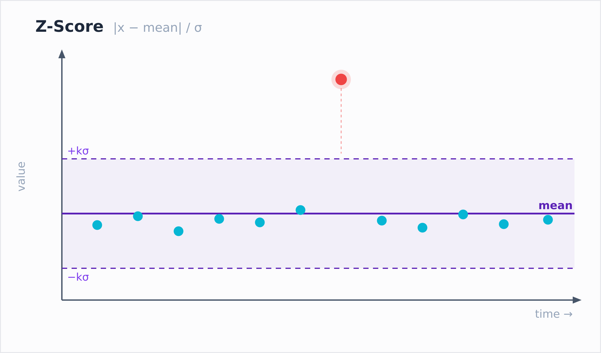Figure 1: Z-Score measures the distance from the mean in units of standard deviationsql

anomaly_score_zscore(value) OVER (window_spec)

Itsminimum valid sample count is 2(it uses the population standard deviation, dividing by n). With fewer than 2 valid points, it returns NULL.

The limitation of Z-Score is that both the mean and the standard deviation are influenced by the outlier itself. A large outlier entering the window pushes up both the mean and the standard deviation, which meansthe outlier dilutes its own anomaly score. You can observe this directly in the full example below: for the same outlier, Z-Score yields a score of about 2, while the other two functions return scores above 100.

When to use it: when the data is fairly clean and stable, and you only need a rough deviation signal, Z-Score is the fastest to compute and good enough.

anomaly_score_mad: more robust for single-point outliers​

MAD stands for Median Absolute Deviation. It replaces the mean in Z-Score with the median, and the standard deviation with MAD:

score = |x − median| / (MAD × 1.4826)

The median is insensitive to outliers—a handful of extreme values barely move the median, yet they shift the mean significantly. This makes MAD far more robust than Z-Score and a better fit for single-point outliers.

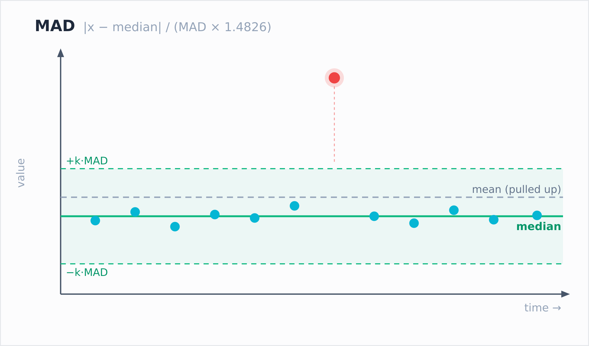Figure 2: An outlier pulls the mean up but leaves the median in place, so MAD stays robustThe1\.4826in the formula is a consistency factor that makes the MAD scoreasymptotically equivalent to the Z-Scorefor normally distributed data. In other words, when the data is clean, MAD and Z-Score produce similar scores; MAD only shows its advantage once outliers are present. The benefit of this design is that you don’t need to recalibrate your threshold when switching between the two functions.

sql

anomaly_score_mad(value) OVER (window_spec)

One detail worth noting: MAD’sminimum valid sample count is 3, one more than Z-Score. The reason is that with only 1–2 samples, MAD is almost always 0, and a MAD of 0 triggers the\+infcase described earlier, producing a flood of meaningless “infinitely anomalous” results. Raising the threshold to 3 is precisely what avoids these spurious alerts.

anomaly_score_iqr: tunable threshold, ideal for alerting​

IQR stands for Interquartile Range, corresponding to the Tukey Fences in statistics. Its idea differs from the first two functions: instead of measuring “how far from the center,” it judges whether a value hascrossed a fence, and by how much.

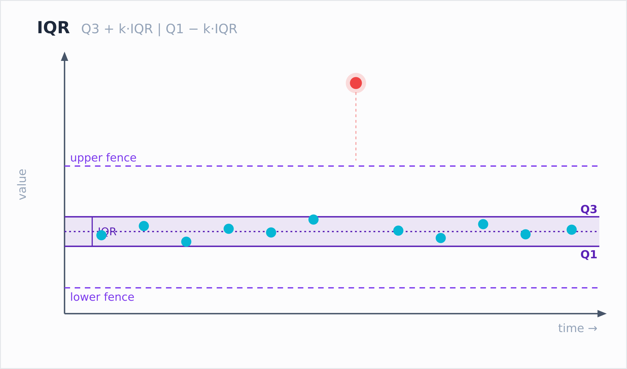Figure 3: IQR builds fences from Q1 and Q3; values inside the fences score exactly 0It takes one more parameter than the other two,k:

sql

anomaly_score_iqr(value, k) OVER (window_spec)

The fences are defined as a lower boundQ1 − k×IQRand an upper boundQ3 \+ k×IQR. The scoring rules are:

• Value below the lower bound:score = \(Q1 − k×IQR − value\) / IQR
• Value above the upper bound:score = \(value − Q3 − k×IQR\) / IQR
• Value within the fences:score = 0\.0

kis a non-negative DOUBLE that controls how tight the fences are.1\.5corresponds to the standard Tukey fences, and3\.0to the looser far-out fences. The largerkis, the more extreme a value must be to get flagged; a negative value makes the function return NULL.

IQR is naturally suited toalerting: every value within the fences scores exactly 0, the boundary is clean, and it won’t assign small fractional scores to normal values the way Z-Score and MAD do. Its minimum valid sample count is also 3 (with linear interpolation, Q1≠Q3 requires at least 3 points).

When to use it: when you want a clear binary “normal / anomalous” boundary and want to control sensitivity by tuningk—for example, start with 1.5, and raise it to 3.0 if alerts are too frequent.

A complete, runnable example​

Below we create a sensor table, write a stretch of stable data, inject a single outlier (80\.0) in the middle, and then apply all three functions at once.

sql

CREATE TABLE sensor_data (
    host   STRING,
    val    DOUBLE,
    ts     TIMESTAMP TIME INDEX,
    PRIMARY KEY (host)
);

INSERT INTO sensor_data VALUES
    ('web-1', 10.0, '2025-01-01 00:00:00'),
    ('web-1', 11.0, '2025-01-01 00:01:00'),
    ('web-1', 10.5, '2025-01-01 00:02:00'),
    ('web-1', 10.8, '2025-01-01 00:03:00'),
    ('web-1', 80.0, '2025-01-01 00:04:00'),  -- outlier
    ('web-1', 10.3, '2025-01-01 00:05:00'),
    ('web-1', 11.2, '2025-01-01 00:06:00');

All three functions share the same window definition. To avoid repeating it, define a single named windowwwith theWINDOWclause, and useROUNDto keep two decimal places for readability:

sql

SELECT
    ts,
    val,
    ROUND(anomaly_score_zscore(val)   OVER w, 2) AS zscore,
    ROUND(anomaly_score_mad(val)      OVER w, 2) AS mad,
    ROUND(anomaly_score_iqr(val, 1.5) OVER w, 2) AS iqr
FROM sensor_data
WINDOW w AS (
    PARTITION BY host
    ORDER BY ts
    ROWS BETWEEN UNBOUNDED PRECEDING AND CURRENT ROW
)
ORDER BY ts;

The output looks like this:

text

+---------------------+------+--------+--------+-------+
| ts                  | val  | zscore | mad    | iqr   |
+---------------------+------+--------+--------+-------+
| 2025-01-01 00:00:00 |   10 |   NULL |   NULL |  NULL |
| 2025-01-01 00:01:00 |   11 |      1 |   NULL |  NULL |
| 2025-01-01 00:02:00 | 10.5 |      0 |      0 |     0 |
| 2025-01-01 00:03:00 | 10.8 |    0.6 |    0.4 |     0 |
| 2025-01-01 00:04:00 |   80 |      2 | 155.58 | 136.5 |
| 2025-01-01 00:05:00 | 10.3 |   0.46 |   0.67 |     0 |
| 2025-01-01 00:06:00 | 11.2 |   0.38 |   0.67 |     0 |
+---------------------+------+--------+--------+-------+

Two details are worth watching.

First,the mad and iqr columns are NULL for the first two rows, while zscore is not. This is the minimum-sample-count difference at work: at the second row (00:01), the window holds only 2 points, which satisfies Z-Score (min=2) but not MAD or IQR (min=3).

Second,for the same outlier (val=80), Z-Score gives only 2, while MAD gives 155.58 and IQR gives 136.5. This confirms the Z-Score self-dilution issue mentioned earlier: the value 80 pushes up both the mean and the standard deviation, so relative to the now-contaminated mean it doesn’t sit that many standard deviations away. MAD and IQR are based on the median and quartiles, which the outlier cannot budge, so they correctly identify the point as strongly anomalous.

The takeaway is clear: to catch single-point outliers, trust MAD or IQR rather than Z-Score.

In practice: filtering anomalous rows directly​

Once you have the scores, what you usually want is not the full score table but the anomalous rows on their own. A window function can’t go directly into aWHEREclause, so wrap the query in a subquery and filter in the outer query:

sql

SELECT * FROM (
    SELECT
        host,
        ts,
        val,
        ROUND(anomaly_score_mad(val) OVER (
            PARTITION BY host
            ORDER BY ts
            ROWS BETWEEN UNBOUNDED PRECEDING AND CURRENT ROW
        ), 2) AS mad
    FROM sensor_data
) WHERE mad > 3.0
ORDER BY host, ts;

Only the anomalous row remains:

text

+-------+---------------------+------+--------+
| host  | ts                  | val  | mad    |
+-------+---------------------+------+--------+
| web-1 | 2025-01-01 00:04:00 |   80 | 155.58 |
+-------+---------------------+------+--------+

The threshold3\.0is a common starting point (roughly matching the intuition of “beyond 3 standard deviations”), but it’s not fixed. Tune it to the noise level of your data.

Choosing the window matters just as much​

Understanding the differences between the three functions matters, but in practice the window range in theOVERclause often has a bigger impact. The example above uses a cumulative window:

sql

ROWS BETWEEN UNBOUNDED PRECEDING AND CURRENT ROW

It accumulates from the start of the series up to the current row. The upside is that the sample grows over time and scores become more stable; the downside is that older data keeps participating in the computation, making it insensitive to slow trend drift.

If your metric has an intraday cycle, or rises overall with each release, asliding windowthat only considers the most recent N points is a better fit:

sql

ROWS BETWEEN 4 PRECEDING AND CURRENT ROW

This way, what counts as “normal” tracks recent data, and older points roll out of the window automatically. Also, don’t dropPARTITION BY host; it ensures each host and each series is computed independently, so one machine’s baseline never gets applied to another.

Summary​

1. **Reach for MAD by default.**Single-point spikes are the most common case in monitoring data, and MAD is the most sensitive to them while being least fooled by the outlier itself.
2. **Use IQR for alert thresholds.**The “0 within the fences” property makes threshold decisions clean, and you can tune sensitivity throughk(try 1.5 first).
3. **Use Z-Score for quick, rough screening.**It works when the data is clean and you only need a coarse signal, but don’t count on it to catch extreme outliers.
4. **Filtering anomalous rows = subquery + outer WHERE.**Window functions can’t go directly into a WHERE clause; one extra layer solves it.
5. **Decide the window first, then pick the function.**A cumulative window favors stability, a sliding window stays close to the recent baseline; always usePARTITION BYto separate different series.

All three functions are purely statistical and detect outliers relative to other points in the window. They don’t do trend forecasting or seasonal anomaly detection, which call for heavier models. But for “a metric suddenly jumps,” the case behind the vast majority of alerts, a single SQL query gets the job done, with no separate data pipeline to maintain.

These three functions are still experimental, and we plan to keep expanding GreptimeDB’s anomaly detection capabilities. If you run into problems or would like to see a particular anomaly detection method, open an issue and let us know:GreptimeTeam/greptimedb Issues.

For the full parameter reference and degenerate-case tables, see the official documentation:Anomaly Detection Functions - GreptimeDB Documentation.