Haskell diagrams: Tessellations

# Haskell diagrams: Tessellations Source: [https://mgarletmilani.com/blog/2026-06-03-tessellations/](https://mgarletmilani.com/blog/2026-06-03-tessellations/) I recently came across some of[Escher](https://en.wikipedia.org/wiki/M._C._Escher)’s impressive and inspiring artworks\. Maybe the[impossible staircase](https://mcescher.com/gallery/most-popular/#iLightbox%5Bgallery_image_1%5D/18)is one of his most famous drawings, but he also worked a lot on[tessellations](https://mcescher.com/gallery/symmetry/)\. A[tessellation](https://en.wikipedia.org/wiki/Tessellation)is the covering of a surface with repeated shapes\. A very familiar type of tessellation is the checkerboard, where the plane is covered with squares of alternating colors\. What makes Escher’s tessellations so fascinating for me is that he managed to cover the plane using birds, fishes, horses or other animals, making an otherwise quite abstract drawing into something alive\. Interestingly, making some form of tessellation is not hard, although it certainly takes an artistic mind to actually find meaningful shapes that fit together\. So let’s reconstruct[one of Escher’s works](https://mcescher.com/gallery/symmetry/#iLightbox%5Bgallery_image_1%5D/59)using Haskell\! If you are not familiar with the`diagrams`library, I recommend reading[my initial post about this library](https://mgarletmilani.com/blog/2026-05-10-penrose-triangle)and[checking the documentation](https://diagrams.github.io/)\. ## Tessellations Let us start with a very basic tessellation: the checkerboard\.  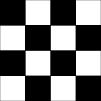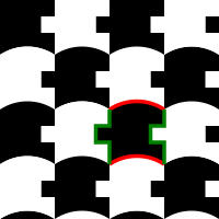How can we modify the squares such that the result still fit? It should be obvious that the left side of the black square must fit the right side of the white square, and the same holds for the top and the bottom sides of the squares\. So if we replace the left and right sides with the same curve, and the top and bottom sides also with the same curve, the resulting tile should fit nicely with its neighbors and cover the whole plane\. To see this, look at the example below\. I marked the left/right sides of one tile in green and the top/bottom sides in red\. As you can see, as long as these lines do not cross, we will obtain a tessellation\.  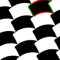Moreover, we do not need to use the same four corners as the square\. As long as the red curve starts where the green curve ends, we can close the boundary and obtain good tile for our tessellation\.  So let us translate this idea into Haskell code\. We use records to specify our tessellations, as they are convenient for storing multiple values of multiples types in one variable\. To make our lives easier, we enable the`OverloadedRecordDot`extension, which lets us write`x\.field`instead of`field x`\. To generate PNG images, we use the`Rasterific`backend, which is available after installing the Haskell library`diagrams\-rasterific`\. ``` {-# LANGUAGE OverloadedRecordDot #-} module Main (main) where -- Hide `intersection` function to avoid a name clash later. import Diagrams.Prelude hiding (intersection) import qualified Diagrams.Backend.Rasterific as Raster ``` There are several data types for curves in`diagrams`\. We will be using`Trail`s, since they are the most convenient type to work with and do exactly what we need\. One nice thing about Haskell’s type system is that it allows us to be very precise\. The sides of our square will be replaced by curves, but not just any curve\. We want open curves, that is, those with loose endpoints\. We express this with the type`Trail' Line V2 a`, where`V2`specifies that we are using two dimensions and`a`is the numeric type we want to use \(we will effectively be using`Double`, but there is no reason to force this now\)\. ``` data ParallelogramTile a = ParallelogramTile { firstSide :: Trail' Line V2 a , secondSide :: Trail' Line V2 a } ``` To create the boundary of one tile, we only need to join the trails together at the endpoints\. The library already gives us convenient functions for this, so our`makeBoundary`function is very straightforward\. ``` -- | The boundary of one tile. makeBoundary :: ParallelogramTile Double -> Trail' Loop V2 Double makeBoundary st = closeLine $ mconcat [ st.firstSide , st.secondSide , (reverseLine st.firstSide) , (reverseLine st.secondSide) ] ``` Observe the difference between the types`Trail' Line V2 Double`and`Trail' Loop V2 Double`\. The type\-system ensures that the output of`makeBoundary`is a*closed*curve, and so we can fill it with color later\. To construct our tile, we will take some measurements from the original image\. This is easy using Inkscape by placing*circles*on top of the points we want to sample\. Just make sure to shift the image so that the origin of the tile is indeed at`\(0,0\)`\. I marked the corners of the parallelogram using yellow dots, the “first” side of the bird with green and the “second” side with red dots\. The yellow dot at the bottom\-left corner is aligned with the`\(0,0\)`coordinate in Inkscape\.  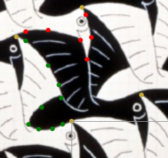We define the curves using[cubic splines](https://en.wikipedia.org/wiki/Cubic_Hermite_spline)\. Cubic splines are very convenient in this context, since they are smooth and go through all specified points\. The only disadvantage is that, if we do not provide enough samples, the curve may get completely out of control and acquire a very bizarre shape\.  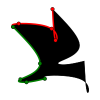This can be easily fixed simply by adding more samples\.  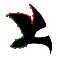After taking enough samples, we can define a bird tile as follows\. The function[`cubicSpline`](https://hackage-content.haskell.org/package/diagrams-lib-1.5.1/docs/Diagrams-CubicSpline.html#v:cubicSpline)takes two arguments: a Boolean value, telling whether the curve should be closed or not, and a list of points\. ``` birdTile = ParallelogramTile { firstSide = cubicSpline False $ map p2 [ (0,0) , (-0.568, 0.2) , (-1.381, 0.4) , (-2.513, 0.472) , (-3.347, 0.078) , (-2.263, -1.323) , (-0.65,-2.089) , (-0.847, -3.168) , (-1.734, -4.762) , (-3.586, -6.793) , (-4.354, -7.116) ] , secondSide = cubicSpline False $ map p2 [ (-4.354, -7.116) , (-3.578, -7.551) , (-1.734, -7.673) , (0.938, -6.851) , (1.467, -5.264) , (1.828, -7.079) , (1.370, -8.939) , (1.057 , -9.545) ] } ``` We can check whether the tile has the correct shape\. 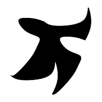``` main :: IO () main = do Raster.renderRasterific "preview.png" (dims $ r2 ( 100 , 100)) (makeBoundary birdTile # stroke # fc black) ```  In case you are wondering why the picture is upside\-down: in Inkscape, the origin`\(0,0\)`is on the top\-left and the y\-axis grows downwards, whereas in`diagrams`\(and in any geometry book I know\) the y\-axis grows upwards\. We can fix this by scaling the y\-axis by`\-1`\. Now we want to cover the entire plane with these birds\. Achieving this takes a couple of steps and some calculations, but everything can be made quite generic such that, if you desire to make your own tessellations, you will not have to think about these auxiliary functions\. For starters, we do not want to draw tiles that will not show up in our image, so we define a function to test if a tile is visible or not\. We test intersections using*bounding boxes*\. A bounding box is an axis\-aligned rectangle which completely contains the desired object \(in our case, our tile\)\. If the bounding box of the tile does not intersect the bounding box of the final view, we know the object is not visible, although the converse is not necessarily true\. Since checking if bounding boxes intersect is very simple and skipping the few extra tiles we might needlessly draw is just not worth the effort, we settle for this approximate solution\. To use bounding boxes, we need to include the`Diagrams\.BoundingBox`module and hide the`intersection`function from the prelude to avoid name clashes\. ``` import Diagrams.BoundingBox ``` Thankfully, the`diagrams`library contains functions for all the calculations we need regarding bounding boxes, so we only need to translate the corners of the bounding box of our tiles\. ``` isTileInsideView :: (BoundingBox V2 Double) -> (P2 Double) -> (BoundingBox V2 Double) -> Bool isTileInsideView tileBox tilePosition viewBox = -- A tile is visible if the intersection -- of its bounding box with the view box -- is not empty. not $ isEmptyBox $ intersection tileBox' viewBox where Just (corner1, corner2) = getCorners tileBox -- Shift the bounding box of the tile to the correct location. -- unP is used to convert a point to a vector. tileBox' = fromCorners (tilePosition .+^ unP corner1) (tilePosition .+^ unP corner2) ``` Next, we need to generate the points on which we will place our tiles\. For this, we use a simple*breadth\-first search*algorithm to explore all visible cells\. Starting at one of the corners of the view bounding box, we look at the*neighboring*cells above, below, to the left and to the right of this corner, and then use`isTileInsideView`above to check if a neighbor is visible or not\. If it is not visible, we do not output it and also do not explore its neighborhood\. Otherwise, if the cell is visible, we output it and also add it to the list of cells whose neighborhood needs to be explored\. To ensure that we do not output cells twice and also that the algorithm terminates, we keep a`Set`of explored cells and only output cells which were not explored yet\. For this, we need the`Set`data structure, which we import by adding the following to the top of our file\. ``` import qualified Data.Set as S ``` If you are familiar with breadth\-first\-search algorithms, the`pointsInsideBox`function below should be very easy to understand\. ``` -- All points corresponding to tiles which -- are visible from the view box. pointsInsideBox :: BoundingBox V2 Double -> BoundingBox V2 Double -- One dimension of the tile. -> V2 Double -- Other dimension of the tile. -> V2 Double -> [((Int, Int), P2 Double)] pointsInsideBox tileBox viewBox v1 v2 = -- Start with (0,0) ((0,0), p0) : pointsInsideBox' (S.singleton (0,0)) [((0,0), p0)] where -- One corner of the view bounding box. p0 = case getCorners viewBox of Just (c0, _) -> c0 Nothing -> error "View bounding box is not defined. Aborting." -- Base case: no more points to explore. pointsInsideBox' explored [] = [] -- Recursive case: There is one point whose -- neighborhood was not explored yet. pointsInsideBox' explored (((r,c), q):active') = -- Output all new points newPoints ++ -- Explore the remaining points. -- The set `explored` contains tiles which -- were already generated. -- This ensures that we do not generate any tile twice. pointsInsideBox' (explored `S.union` (S.fromList $ map fst newPoints)) (newPoints ++ active') where newPoints = filter (\((r',c'), q') -> isTileInsideView tileBox q' viewBox && (not ((r', c') `S.member` explored))) [ ((r+1,c), q .+^ v1) -- Right , ((r-1,c), q .-^ v1) -- Left , ((r,c-1), q .-^ v2) -- Bottom , ((r,c+1), q .+^ v2) -- Top ] ``` To generate the visible cells, all we have to do now is compute the bounding boxes and the`v1`and`v2`vectors above telling where the neighboring tiles should lie\. Thankfully,`diagrams`provides a`boundingBox`function which computes the bounding box of any diagram, so the`gridPoints`function below only needs to tie all the functions together\. ``` gridPoints :: ParallelogramTile Double -> Double -> Double -> [((Int, Int), P2 Double)] gridPoints tile width height = pointsInsideBox tileBox viewBox v1 v2 where -- Bounding box of a tile positioned at (0,0). tileBox = (boundingBox $ makeBoundary tile) -- Bounding box of the view. viewBox = (fromCorners (p2 (0,0)) (p2 (width, height))) -- The two vectors corresponding to the sides of the tile. v1 = (tile.firstSide `atParam` domainUpper tile.firstSide) .-. (tile.firstSide `atParam` domainLower tile.firstSide) v2 = (tile.secondSide `atParam` domainUpper tile.secondSide) .-. (tile.secondSide `atParam` domainLower tile.secondSide) ``` If we try to generate the grid now, we will have a rather boring image, as all tiles have the same color and so we are just filling the entire screen with one color\. To make the picture more lively, I will choose green and yellow as colors for the tiles\. The birds also have eyes, feathers, a beak and other details\. We will define`birdDecorations`later\. For now, we just use a dummy function\. ``` birdDecorations _ _ = mempty ``` We will color the tiles based on their row and column along the grid\. Obtaining a checkerboard pattern from this is very easy\. ``` colors = [green, yellow] bird (row, column) = mconcat [ birdDecorations primary secondary , makeBoundary birdTile # stroke # fc primary # lc primary -- Add a very thin line to avoid artifacts when rendering. # lw 0.0001 ] where index = ((row + column) `mod` 2) primary = colors !! index secondary = colors !! (1 - index) ``` We can now preview how the tiles fit together\. ``` dia viewW viewH = -- Position the tiles. (position $ map (\(cell, v) -> (v, bird cell)) (gridPoints birdTile viewW viewH)) -- Only show tiles inside the view box. # clipTo ( pathFromTrail $ wrapTrail $ closeLine $ lineFromVertices $ [ p2 (0,0) , p2 (0, viewH) , p2 (viewW, viewH) , p2 (viewW, 0) ]) -- Invert y-axis because we used Inkscape coordinates. # scaleY (-1) main :: IO () main = do let width = 35 :: Double height = 35 resolution = 8 Raster.renderRasterific "tessellation.png" (dims $ r2 ( width * resolution , height * resolution)) (dia width height) ``` To render the image, we only need to call`runhaskell Tessellation\.hs`, and this will generate the PNG image\.  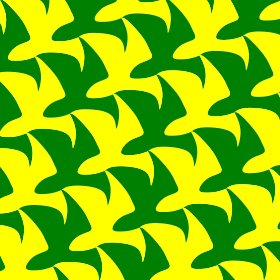Without the details, however, the birds are not recognizable as such\. Using a program such as Inkscape as a helper, we can obtain the coordinates we need to add the details to the birds\. One important point to observe here is the usage of`local`for the thickness of the lines\. In diagrams, using a*local measurement*means that the actual thickness will be determined relative to the final dimensions used\. If we just use`0\.1`instead, the lines will become thicker or thinner depending on the dimensions of our image, which, in this case, is undesirable\. ``` wingDetail = local 0.1 birdEye primary secondary = mconcat [ circle 0.15 # fc primary # lw 0 , circle 0.3 # fc secondary # lc primary # lw (local 0.1) ] birdDecorations primary secondary = position -- Eye [ ( p2 (5.503, -1.323) , birdEye primary secondary) -- Front wing, lower part , ( p2 (1.544, -1.099) , cubicSpline False [ p2 (1.544, -1.099) , p2 (0.179, -1.323) , p2 (-0.65, -2.389) ] # strokeTrail # lw wingDetail # lc secondary ) -- Front wing, feathers , ( p2 (-2.8, -6.75) , arcBetween (p2 (0,0)) (p2 (2.5,0.2)) (-0.15) # lw wingDetail # lc secondary ) , ( p2 (-1.75, -5.55) , arcBetween (p2 (0,0)) (p2 (1.5,-0.1)) (-0.15) # lw wingDetail # lc secondary ) , ( p2 (-1.05, -4.3) , arcBetween (p2 (0,0)) (p2 (1.2,-0.25)) (-0.12) # lw wingDetail # lc secondary ) , ( p2 (-0.6, -3.2) , arcBetween (p2 (0,0)) (p2 (0.9,-0.3)) (-0.08) # lw wingDetail # lc secondary ) , ( p2 (-0.1, -2.1) , arcBetween (p2 (0,0)) (p2 (0.8,-0.6)) (-0.05) # lw wingDetail # lc secondary ) , ( p2 (0.75, -1.3) , arcBetween (p2 (0,0)) (p2 (0.5,-0.7)) (-0.04) # lw wingDetail # lc secondary ) -- Between front and back wings , ( p2 (2.439, -1.486) , cubicSpline False [ p2 (2.439, -1.486) , p2 (1.807, -2.115) , p2 (1.666, -4.457) , p2 (1.48, -5.4) ] # strokeTrail # lw wingDetail # lc secondary ) -- Feathers on back wing , ( p2 (1.85, -8.2) , arcBetween (p2 (0,0)) (p2 (1.2, 0.8)) (-0.15) # lw wingDetail # lc secondary ) , ( p2 (2.0, -7.0) , arcBetween (p2 (0,0)) (p2 (1, 0.75)) (-0.15) # lw wingDetail # lc secondary ) , ( p2 (1.8, -5.9) , arcBetween (p2 (0,0)) (p2 (0.8, 0.6)) (-0.1) # lw wingDetail # lc secondary ) , ( p2 (1.62, -4.9) , arcBetween (p2 (0,0)) (p2 (0.8, 0.55)) (-0.05) # lw wingDetail # lc secondary ) , ( p2 (1.65, -3.8) , arcBetween (p2 (0,0)) (p2 (0.6, 0.4)) (-0.05) # lw wingDetail # lc secondary ) -- Beak , ( p2 (6.204, -0.763) , cubicSpline False [ p2 (6.204, -0.763) , p2 (5.882, -0.458) , p2 (5.36, -0.508) , p2 (5.36, 0.45) ] # strokeTrail # lw wingDetail # lc secondary ) ] ``` We now obtain the following\.  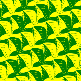I like the pattern so much, I also want to have a wallpaper version of it\. For this, I only need to add this to the end of`main`\. ``` Raster.renderRasterific "tessellation-escher-1-wallpaper-1080p.png" (dims $ r2 (1920, 1080)) (dia (19.2 * 6) (10.8 * 6)) ``` If you need higher resolution, just change the`1920`and`1080`values there\. ## Conclusion Tessellations are quite amusing drawings\. While the code here might be a bit long and it might take some time to do all the calculations, it is quite generic \(for parallelogram\-based tessellations\)\. If you want to play around and make your own tessellations, you only need to define a value of type`ParallelogramTessellation Double`and replace the`bird`function with your own\. To make things more ergonomic, I turned the code above into a`Diagrams\.TwoD\.Tessellation`module in this[git repository](https://gitlab.com/mgmillani/diagrams-gallery)\. While drawing complex curves like the tile decorations above programmatically is certainly more cumbersome than using a GUI application such as Inkscape, using a library like diagrams allows us to separate the artistic part from the technical, computational task of properly assembling the tiles and positioning them\. Moreover, while writing the code above, I felt it was rather straightforward to organize the functions in a modular way\. Extracting them into a module was not time consuming\. Even if I had any idea how to achieve this using TikZ \(which I don’t\), the result would not be something I would try to put in its own package\. I will continue my journey of exploring the`diagrams`library\. Hopefully, my next project will not just be something amusing, but also something I can use in my work\.