This article explains the fundamentals of Markov Decision Processes (MDPs), a core framework in deep reinforcement learning, using an educational example of a student's daily decisions.
<p><em>by Surya Vengadesan</em></p><p>With deep reinforcment learning’s success in beating humans at games including Go, Dota 2, and even Poker, there is a lot of excitement around the field and people want to understand its algorithms from the ground up. In this blog post, we will do just that. We will explore a fundamental building block of deep RL: Markov Decision Processess — a framework that models how an agent behaves and learns from it’s environment. In particular, we will lay out the theory of MDPs and explore approximate methods for solving them.</p><h3>Mr. Markov Navigating College</h3><p>Now, let’s walk through MDPs by studying a specific agent. Specifically, an agent is an entity that interacts within its environment and interatively learns how to best act within the environment. For our example, Mr. Markov will be our agent; he is an undergraduate studying mathematics. Markov needs to make many decisions while in college (his environment). In a typical day, Markov studies for his probability theory class, sleeps in his bed, or socializes with his friends in hour long chunks. Markov is faced with a problem. Some days Markov is incredibly tired from staying up to finish his problem sets or feels stir-crazy from sitting at his desk for hours on end. Therefore, Markov needs a process to help him navigate through his daily decisions in hopes to bring him peace.</p><h3>Modeling Mr. Markov’s World</h3><p>In this blog post we are going to help this poor student, by laying out a Markov Decision Process to model his world, then figure out what actions he should take in his best self-interest. Markov, at any given time, could be in one of a finite number of states. Let’s denote these in a set called the state space:</p><div class="latex-rendered" data-attrs="{"persistentExpression":"\\mathcal{S} = \\{s_1 \\text{ (studying)}, s_2 \\text{ (sleeping)}, s_3 \\text{ (socializing)}\\}","id":"FAFEUMTRQO"}" data-component-name="LatexBlockToDOM"></div><p>In addition, in any given state he could decide from a set of actions. Let’s denote these in a set called the action space:</p><div class="latex-rendered" data-attrs="{"persistentExpression":"\\mathcal{A} = \\{a_1 \\text{ (message a friend)}, a_2 \\text{ (read Tolstoy)}, a_3 \\text{ (eat a snack)}\\}","id":"KJWELGPETJ"}" data-component-name="LatexBlockToDOM"></div><p>In our model world, at every hour, Markov can perform one of these three actions from any of the three states. We shall demarcate these hours of the day by variable ttt. By taking an action at a specific state at a specific time <em>t</em>, Markov will end up in a new state s′∈S. We shall also define a set of non-negative probabilities for each state-action pair and it’s resulting action, P(s′∣s,a)≥0, and with any probability distribution these must add to 1: Σs′ P(s′∣s,a)=1.</p><p>Now, we ask Markov a question: “What is your purpose? What do you value?.” Markov, an aspiring future graduate student in mathematics, responds, “To one day teach probability theory to other students and perform original research within the field.” To help this aspiring future probability theorist, let’s add a few more definitions to his decision-making framework, that can help quantify what he values. For each state-action pair and associated next state, we assign a scalar reward r(s′∣s,a)=c. We ask Markov a follow up question: “What’s your plan? How do you plan on getting into graduate school?” He responds, “I’m going to study, study a lot.” Now, to help Markov on his journey, we add a few extra formalisms. First we formalize his <em>plan</em> into a function, and call it a policy function π(a∣s) that maps every state with a specific action to take.</p><p>To sum it up, say he’s in state <em>s<sub>1</sub></em>=studying, and he decided to take the action of <em>a<sub>1</sub></em>=messaging a friend according to his policy. Given <em>(s<sub>1</sub>,a<sub>1</sub>)</em>, he now has the following probabilities at ending up the following states after completing the action, </p><div class="latex-rendered" data-attrs="{"persistentExpression":"t(s_1 (\\text{studying})| s_1, a_1) = 0.2","id":"MKQMTTSVIK"}" data-component-name="LatexBlockToDOM"></div><div class="latex-rendered" data-attrs="{"persistentExpression":"t(s_2 (\\text{sleeping})|s_1, a_1) = 0.2","id":"KTNFJQIPRL"}" data-component-name="LatexBlockToDOM"></div><div class="latex-rendered" data-attrs="{"persistentExpression":"t(s_3 (\\text{socializing})|s_1, a_1) = 0.6","id":"WYYONKJWUQ"}" data-component-name="LatexBlockToDOM"></div><p>which add up to 1 as defined previously. Let’s also define a set of rewards that we believe best align with what Markov says he values. We can assign real values rewards to each state he next ends up in after performing action <em>a<sub>1</sub></em> in state <em>s<sub>1</sub></em>, </p><div class="latex-rendered" data-attrs="{"persistentExpression":"r(s_1(\\text{studying})|s_1, a_1) = 10","id":"HCYIOZNUTP"}" data-component-name="LatexBlockToDOM"></div><div class="latex-rendered" data-attrs="{"persistentExpression":"r(s_2(\\text{sleeping})|s_1, a_1) = 5","id":"YRHARZVITC"}" data-component-name="LatexBlockToDOM"></div><div class="latex-rendered" data-attrs="{"persistentExpression":"r(s_3(\\text{socializing})|a_1, s_1) = 3","id":"MCATMIJIVQ"}" data-component-name="LatexBlockToDOM"></div><p>Together, we have incorporated stochastic behavior and measures of value and into the framework, since each state-action pair is now mapped to a probability distribution and a set of rewards that uniquely determine each next possible state. In essence, we have just laid out the mathematical formalism for MDPs, which not only helps Markov, but more generally exists as a tool that lies at the core of many control theory applications, including reinforcement learning.</p><h3>Recap of Definitions</h3><p>We have defined 4 quantities making up the tuple <S,A,T,R>, which includes a state space, an action space, a transition function, and a reward function. In our specific example with Markov, we have 3 states, 3 rewards, and a transition and reward function that map all pairs of state-action transitions (s’|a, s) with an associated probability reward, totalling to 27 scalars each. What we have just defined above, is referred to as a <em>finite</em> MDP, because element of the tuple consists of finite sets. Below is a subset of the MDP over an arbitrary state action pair (s<sub>i</sub>,a<sub>i</sub>).</p><div class="captioned-image-container"><figure><a class="image-link image2 is-viewable-img" target="_blank" href="https://substackcdn.com/image/fetch/$s_!z7ER!,f_auto,q_auto:good,fl_progressive:steep/https%3A%2F%2Fsubstack-post-media.s3.amazonaws.com%2Fpublic%2Fimages%2Fc1fb9784-e12a-45eb-bf9e-c28ce1a9bf6e_547x354.png" data-component-name="Image2ToDOM"><div class="image2-inset"><picture><source type="image/webp" srcset="https://substackcdn.com/image/fetch/$s_!z7ER!,w_424,c_limit,f_webp,q_auto:good,fl_progressive:steep/https%3A%2F%2Fsubstack-post-media.s3.amazonaws.com%2Fpublic%2Fimages%2Fc1fb9784-e12a-45eb-bf9e-c28ce1a9bf6e_547x354.png 424w, https://substackcdn.com/image/fetch/$s_!z7ER!,w_848,c_limit,f_webp,q_auto:good,fl_progressive:steep/https%3A%2F%2Fsubstack-post-media.s3.amazonaws.com%2Fpublic%2Fimages%2Fc1fb9784-e12a-45eb-bf9e-c28ce1a9bf6e_547x354.png 848w, https://substackcdn.com/image/fetch/$s_!z7ER!,w_1272,c_limit,f_webp,q_auto:good,fl_progressive:steep/https%3A%2F%2Fsubstack-post-media.s3.amazonaws.com%2Fpublic%2Fimages%2Fc1fb9784-e12a-45eb-bf9e-c28ce1a9bf6e_547x354.png 1272w, https://substackcdn.com/image/fetch/$s_!z7ER!,w_1456,c_limit,f_webp,q_auto:good,fl_progressive:steep/https%3A%2F%2Fsubstack-post-media.s3.amazonaws.com%2Fpublic%2Fimages%2Fc1fb9784-e12a-45eb-bf9e-c28ce1a9bf6e_547x354.png 1456w" sizes="100vw"><img src="https://substackcdn.com/image/fetch/$s_!z7ER!,w_1456,c_limit,f_auto,q_auto:good,fl_progressive:steep/https%3A%2F%2Fsubstack-post-media.s3.amazonaws.com%2Fpublic%2Fimages%2Fc1fb9784-e12a-45eb-bf9e-c28ce1a9bf6e_547x354.png" width="547" height="354" data-attrs="{"src":"https://substack-post-media.s3.amazonaws.com/public/images/c1fb9784-e12a-45eb-bf9e-c28ce1a9bf6e_547x354.png","srcNoWatermark":null,"fullscreen":null,"imageSize":null,"height":354,"width":547,"resizeWidth":null,"bytes":null,"alt":null,"title":null,"type":null,"href":null,"belowTheFold":true,"topImage":false,"internalRedirect":null,"isProcessing":false,"align":null,"offset":false}" class="sizing-normal" alt="" srcset="https://substackcdn.com/image/fetch/$s_!z7ER!,w_424,c_limit,f_auto,q_auto:good,fl_progressive:steep/https%3A%2F%2Fsubstack-post-media.s3.amazonaws.com%2Fpublic%2Fimages%2Fc1fb9784-e12a-45eb-bf9e-c28ce1a9bf6e_547x354.png 424w, https://substackcdn.com/image/fetch/$s_!z7ER!,w_848,c_limit,f_auto,q_auto:good,fl_progressive:steep/https%3A%2F%2Fsubstack-post-media.s3.amazonaws.com%2Fpublic%2Fimages%2Fc1fb9784-e12a-45eb-bf9e-c28ce1a9bf6e_547x354.png 848w, https://substackcdn.com/image/fetch/$s_!z7ER!,w_1272,c_limit,f_auto,q_auto:good,fl_progressive:steep/https%3A%2F%2Fsubstack-post-media.s3.amazonaws.com%2Fpublic%2Fimages%2Fc1fb9784-e12a-45eb-bf9e-c28ce1a9bf6e_547x354.png 1272w, https://substackcdn.com/image/fetch/$s_!z7ER!,w_1456,c_limit,f_auto,q_auto:good,fl_progressive:steep/https%3A%2F%2Fsubstack-post-media.s3.amazonaws.com%2Fpublic%2Fimages%2Fc1fb9784-e12a-45eb-bf9e-c28ce1a9bf6e_547x354.png 1456w" sizes="100vw" loading="lazy"></picture><div class="image-link-expand"><div class="pencraft pc-display-flex pc-gap-8 pc-reset"><button tabindex="0" type="button" class="pencraft pc-reset pencraft icon-container restack-image"><svg role="img" width="20" height="20" viewBox="0 0 20 20" fill="none" stroke-width="1.5" stroke="var(--color-fg-primary)" stroke-linecap="round" stroke-linejoin="round" xmlns="http://www.w3.org/2000/svg"><g><title></title><path d="M2.53001 7.81595C3.49179 4.73911 6.43281 2.5 9.91173 2.5C13.1684 2.5 15.9537 4.46214 17.0852 7.23684L17.6179 8.67647M17.6179 8.67647L18.5002 4.26471M17.6179 8.67647L13.6473 6.91176M17.4995 12.1841C16.5378 15.2609 13.5967 17.5 10.1178 17.5C6.86118 17.5 4.07589 15.5379 2.94432 12.7632L2.41165 11.3235M2.41165 11.3235L1.5293 15.7353M2.41165 11.3235L6.38224 13.0882"></path></g></svg></button><button tabindex="0" type="button" class="pencraft pc-reset pencraft icon-container view-image"><svg xmlns="http://www.w3.org/2000/svg" width="20" height="20" viewBox="0 0 24 24" fill="none" stroke="currentColor" stroke-width="2" stroke-linecap="round" stroke-linejoin="round" class="lucide lucide-maximize2 lucide-maximize-2"><polyline points="15 3 21 3 21 9"></polyline><polyline points="9 21 3 21 3 15"></polyline><line x1="21" x2="14" y1="3" y2="10"></line><line x1="3" x2="10" y1="21" y2="14"></line></svg></button></div></div></div></a></figure></div><p>Using this structure, we would like to figure out what actions we should take to get the highest reward; fortunately, there exist proven algorithms to do exactly this. We will soon attempt to solve for an optimal policy function π(⋅) using said algorithms in Markov’s world. Through our specific example, we are attempting to solve the old, and suprisingly relevant meme (below), but with extreme precision due to the beauty of finite MDPs.</p><div class="captioned-image-container"><figure><a class="image-link image2 is-viewable-img" target="_blank" href="https://substackcdn.com/image/fetch/$s_!npko!,f_auto,q_auto:good,fl_progressive:steep/https%3A%2F%2Fsubstack-post-media.s3.amazonaws.com%2Fpublic%2Fimages%2Fe36f205a-e89e-4f0b-9fc1-a66cb6509512_500x397.png" data-component-name="Image2ToDOM"><div class="image2-inset"><picture><source type="image/webp" srcset="https://substackcdn.com/image/fetch/$s_!npko!,w_424,c_limit,f_webp,q_auto:good,fl_progressive:steep/https%3A%2F%2Fsubstack-post-media.s3.amazonaws.com%2Fpublic%2Fimages%2Fe36f205a-e89e-4f0b-9fc1-a66cb6509512_500x397.png 424w, https://substackcdn.com/image/fetch/$s_!npko!,w_848,c_limit,f_webp,q_auto:good,fl_progressive:steep/https%3A%2F%2Fsubstack-post-media.s3.amazonaws.com%2Fpublic%2Fimages%2Fe36f205a-e89e-4f0b-9fc1-a66cb6509512_500x397.png 848w, https://substackcdn.com/image/fetch/$s_!npko!,w_1272,c_limit,f_webp,q_auto:good,fl_progressive:steep/https%3A%2F%2Fsubstack-post-media.s3.amazonaws.com%2Fpublic%2Fimages%2Fe36f205a-e89e-4f0b-9fc1-a66cb6509512_500x397.png 1272w, https://substackcdn.com/image/fetch/$s_!npko!,w_1456,c_limit,f_webp,q_auto:good,fl_progressive:steep/https%3A%2F%2Fsubstack-post-media.s3.amazonaws.com%2Fpublic%2Fimages%2Fe36f205a-e89e-4f0b-9fc1-a66cb6509512_500x397.png 1456w" sizes="100vw"><img src="https://substackcdn.com/image/fetch/$s_!npko!,w_1456,c_limit,f_auto,q_auto:good,fl_progressive:steep/https%3A%2F%2Fsubstack-post-media.s3.amazonaws.com%2Fpublic%2Fimages%2Fe36f205a-e89e-4f0b-9fc1-a66cb6509512_500x397.png" width="500" height="397" data-attrs="{"src":"https://substack-post-media.s3.amazonaws.com/public/images/e36f205a-e89e-4f0b-9fc1-a66cb6509512_500x397.png","srcNoWatermark":null,"fullscreen":null,"imageSize":null,"height":397,"width":500,"resizeWidth":null,"bytes":null,"alt":null,"title":null,"type":null,"href":null,"belowTheFold":true,"topImage":false,"internalRedirect":null,"isProcessing":false,"align":null,"offset":false}" class="sizing-normal" alt="" srcset="https://substackcdn.com/image/fetch/$s_!npko!,w_424,c_limit,f_auto,q_auto:good,fl_progressive:steep/https%3A%2F%2Fsubstack-post-media.s3.amazonaws.com%2Fpublic%2Fimages%2Fe36f205a-e89e-4f0b-9fc1-a66cb6509512_500x397.png 424w, https://substackcdn.com/image/fetch/$s_!npko!,w_848,c_limit,f_auto,q_auto:good,fl_progressive:steep/https%3A%2F%2Fsubstack-post-media.s3.amazonaws.com%2Fpublic%2Fimages%2Fe36f205a-e89e-4f0b-9fc1-a66cb6509512_500x397.png 848w, https://substackcdn.com/image/fetch/$s_!npko!,w_1272,c_limit,f_auto,q_auto:good,fl_progressive:steep/https%3A%2F%2Fsubstack-post-media.s3.amazonaws.com%2Fpublic%2Fimages%2Fe36f205a-e89e-4f0b-9fc1-a66cb6509512_500x397.png 1272w, https://substackcdn.com/image/fetch/$s_!npko!,w_1456,c_limit,f_auto,q_auto:good,fl_progressive:steep/https%3A%2F%2Fsubstack-post-media.s3.amazonaws.com%2Fpublic%2Fimages%2Fe36f205a-e89e-4f0b-9fc1-a66cb6509512_500x397.png 1456w" sizes="100vw" loading="lazy"></picture><div class="image-link-expand"><div class="pencraft pc-display-flex pc-gap-8 pc-reset"><button tabindex="0" type="button" class="pencraft pc-reset pencraft icon-container restack-image"><svg role="img" width="20" height="20" viewBox="0 0 20 20" fill="none" stroke-width="1.5" stroke="var(--color-fg-primary)" stroke-linecap="round" stroke-linejoin="round" xmlns="http://www.w3.org/2000/svg"><g><title></title><path d="M2.53001 7.81595C3.49179 4.73911 6.43281 2.5 9.91173 2.5C13.1684 2.5 15.9537 4.46214 17.0852 7.23684L17.6179 8.67647M17.6179 8.67647L18.5002 4.26471M17.6179 8.67647L13.6473 6.91176M17.4995 12.1841C16.5378 15.2609 13.5967 17.5 10.1178 17.5C6.86118 17.5 4.07589 15.5379 2.94432 12.7632L2.41165 11.3235M2.41165 11.3235L1.5293 15.7353M2.41165 11.3235L6.38224 13.0882"></path></g></svg></button><button tabindex="0" type="button" class="pencraft pc-reset pencraft icon-container view-image"><svg xmlns="http://www.w3.org/2000/svg" width="20" height="20" viewBox="0 0 24 24" fill="none" stroke="currentColor" stroke-width="2" stroke-linecap="round" stroke-linejoin="round" class="lucide lucide-maximize2 lucide-maximize-2"><polyline points="15 3 21 3 21 9"></polyline><polyline points="9 21 3 21 3 15"></polyline><line x1="21" x2="14" y1="3" y2="10"></line><line x1="3" x2="10" y1="21" y2="14"></line></svg></button></div></div></div></a></figure></div><p>Before, we reach the solution, however, we need a few more tools defined below.</p><h3>More Fun Functions</h3><p>Given these well defined transition dynamics and rewards of Markov’s model world, we can define two additional functions. The first is the state-value function. This is determined by the state Markov is currently in and also his current policy function:</p><div class="latex-rendered" data-attrs="{"persistentExpression":"v_\\pi(s) = \\mathbb{E}_\\pi[\\Sigma_{k=0}^\\infty \\gamma^kR_{t+k+1}|S_t=s]","id":"AUUCVCFQVG"}" data-component-name="LatexBlockToDOM"></div><p>This can be interpreted as the long-term expected reward that Markov will receive from currently being in state sss and acting according to his plan. Here, we have two random variables that <em>S<sub>t</sub></em> and <em>R<sub>t</sub></em> that model the state and reward the agent will be in and recieve, at time step <em>t</em>, if it follows the policy defined by π(⋅). We have also introduced a new variable γ which we call the discount rate, that can be any value from 0≤γ≤1. The term in the expectation expands out to this form:</p><div class="latex-rendered" data-attrs="{"persistentExpression":"\\gamma^k R_{t+k+1} = \\gamma^0 R_1 + \\gamma^1 R_2 + \\gamma^2 R_3 + \\cdots","id":"JNLPOXITDY"}" data-component-name="LatexBlockToDOM"></div><p>In essence, the value of the reward gained by taking an action and landing in a new state in the future, is being reduced by a multiple of γ with each time step that passes. This answers the question on how much a given reward is depriciated each ttt time step into the future, before it has been obtained.</p><p>Altogether, the state-value function <em>v<sub>π</sub></em>(⋅) allows us to help Markov gauge the <em>value</em> he obtains from his tentative <em>plan</em> that we have formalized by the policy function <em>π(⋅)</em>. Now, the curious Markov asks us, “Well, assume I’m working on my probability pset and decide to go read War and Peace by Leo Tolstoy, is that a good idea?” To answer this, let’s add our final function to put Markov’s mind at rest. Let’s call it the action-value function <em>q<sub>π</sub>(s,a)</em>, which is the expected return in rewards he receives, computed similarly to the state-value function, but incorporating the reward from an initial action aaa instead of action <em>π(s)</em>:</p><div class="latex-rendered" data-attrs="{"persistentExpression":"q_\\pi(s, a) = \\mathbb{E}_\\pi[\\Sigma_{k=0}^\\infty \\gamma^k R_{t+k+1} | S_t = s, A_t = a]","id":"VSYLHTARUW"}" data-component-name="LatexBlockToDOM"></div><p>This seemingly insignificant distinction will help us when it comes time to compute the optimal policy π<em><sup>*</sup></em>(⋅). Together, the state-value and action-value functions, are called the Bellman equations. We, will now solve for the value of these Bellman equations at each state or state-action pair, using two fundamental algorithms.</p><h3>Solving via Policy Iteration</h3><p>The first main algorithm used to solve finite MDPs is called Policy Iteration. This algorithm iterates between two steps. The first step is to evaluate the value function for all states of an MDP given an arbitrary policy. This is commonly referred to as <em>policy evaluation</em>. The second step is to consider for each state, whether taking action a≠π(s) (not part of the policy) can improve the overall expected return. This is commonly referred to as <em>policy evaluation</em>. The algorithm loops through these steps, finding a better policy at each iteration until convergence.</p><p>Now, we shall implement Markov’s model world using python and numpy. We follow the standard algorithm implementation outlined in Richard Sutton’s RL <a href="http://incompleteideas.net/book/first/ebook/node40.html">textbook</a>. However, we make a few simplificiations for a quick build. (1) Our model only has 1 reward per (s’, s, a) pairs, while others allow for a distribution over rewards (2) We are searching to solve for a deterministic policy, while others can solve for a stochastic policy (3) Instead of defining 56 carefully engineered rewards and transitions, we assign fixed values (4) To assure convergence of our expected long term reward (to avoid values approaching infinity), so we include a discount rate of 0.85.</p><p>We first need to make a few imports and initialize our finite MDP.</p><pre><code>import numpy as np
import matplotlib.pyplot as plt
import math
states = 3 #Number of States
actions = 3 #Number of Actions
rewards = 3 #Number of Rewards per State-action Pair
g = 0.85 #Discount Rate - gamma
v_s = [0, 0, 0] #State-value Function
pi = [0, 0, 0] #Deterministic Policy Function
theta = 1 #Hyperparameter
np.random.seed(0) #Random seed used to initalize Reward Function
R = 100 * np.random.rand(3, 3, 3) #Reward Function: intialize a 3x3x3 tensor of random values from 0 to 100
T = np.full((3,3,3), 1/3) #Transition Function: intialize a 3x3x3 tensor of 1/3s
PI = [] #List to keep track of value function for Policy Iteration
VI = [] #List to keep track of value function for Value Iteration
print(R) #Our specific Reward Function
#Randomly Initialized Reward Function
[[[54.88135039 71.51893664 60.27633761]
[54.4883183 42.36547993 64.58941131]
[43.75872113 89.17730008 96.36627605]]
[[38.34415188 79.17250381 52.88949198]
[56.80445611 92.55966383 7.10360582]
[ 8.71292997 2.02183974 83.26198455]]
[[77.81567509 87.00121482 97.86183422]
[79.91585642 46.14793623 78.05291763]
[11.82744259 63.99210213 14.33532874]]]</code></pre><p>Now for the implementation of Policy Iteration, which initializes an arbitraty policy and state-value function, then iterates between policy evaluation and policy improvement stages.</p><pre><code>def policy_iteration(pol, val, thres):
#Initialize Policy and Value Function
policy = pol
threshold = thres
v_s_init = val
PI.append(v_s_init.copy())
#Run first iteration of PE to evaluate your arbitrary policy
value = policy_evaluation(pi, v_s_init, threshold)
PI.append(value.copy())
#Run first iteration of PI to find actions that might prove it
policy_stable, policy = policy_improvement(pi, value)
#Repeat PE and PI, until no change in policy improves performance (i.e. policy_stable = True)
while policy_stable == False:
value = policy_evaluation(policy, value, threshold)
PI.append(value.copy())
policy_stable, policy = policy_improvement(policy, value)
return policy, value
def policy_evaluation(pol, val, thres):
policy = pol
threshold = thres
v_s_init = val
delta = math.inf
#Evalute accuracy until Delta drops below specified threshold value
while delta >= threshold:
delta = 0
#Compute expected return for each state, given the current policy
for s in range(states):
v = v_s_init[s]
E_r = 0
for s_p in range(states):
E_r += T[s, policy[s], s_p]*(R[s, policy[s], s_p] + g*v_s_init[s_p])
v_s_init[s] = E_r
delta = max(delta, abs(v - v_s_init[s]))
return v_s_init
def policy_improvement(pol, val):
policy_stable = True
policy = pol.copy()
v_s_init = val
for s in range(states):
old_a = pol[s]
v = v_s_init[s]
E_r = []
#Evalute expected value of each state and action pair
for a in range(actions):
e_r = 0
for s_p in range(states):
e_r += T[s, a, s_p]*(R[s, a, s_p] + g*v_s_init[s_p])
E_r.append(e_r)
#Select action the maximizes expected value
new_a = E_r.index(max(E_r))
#Compare if action that maximizes expected value is action specified by current policy
if(old_a != new_a):
#If not, modify policy and report stability to false, to ensure PI evalutes new policy
policy[s] = new_a
policy_stable = False
return policy_stable, policy
#Run Algorithm
new_pi, new_v = value_iteration(pi, v_s, theta)</code></pre><p>Algorithm Output: </p><div class="latex-rendered" data-attrs="{"persistentExpression":"v_{\\pi*}(s_1, s_2, s_3) = [489.98445020171096, 470.622736297478, 501.629766335168]","id":"UHSNHGMZUH"}" data-component-name="LatexBlockToDOM"></div><div class="latex-rendered" data-attrs="{"persistentExpression":"\\pi_*(s_1, s_2, s_3) = [2, 0, 0]","id":"LZRHQSKFGD"}" data-component-name="LatexBlockToDOM"></div><p>By running this algorithm, we obtain the optimal state-value function and optimal policy shown above. Now this example is clearly idealistic, we are given the states, actions, and rewards. In the real world we don’t have this, and real world problems are typically much more complicated. Figuring out how to solve more complex, obscure problems is an open challenge that the field faces to this day. In short, MDPs solve real-world problems only as best as you can model problems in the first place. Therefore, although we may not be able gaurantee that our policy will help Markov in the real-world, we hope that the theoretical implications can provide insight into his decision making.</p><h3>Solving via Value Iteration and More</h3><p>Now, let’s attempt to find the optimal policy of out student’s Markov’s work using Value Iteration. The structure of this algorithm is very similar to Policy Iteration, but differs slightly. Instead of iterating back and forth between improvement and evaluation in Policy Iteration, Value Iteration performs a single iteration of a pseudo policy evaluation, where it additionally sweeps over the action space and perform a max operation to return the optimal state-value function and policy function upon completion.</p><pre><code>def value_iteration(pol, val, thres):
#Initialize Policy and Value Function
policy = pol
threshold = thres
v_s_init = val
VI.append(v_s_init.copy())
delta = math.inf
#Loop until delta reaches specified threshold
while delta >= threshold:
delta = 0
#Evalute expected value of each state and action pair
for s in range(states):
v = v_s_init[s]
E_r = []
for a in range(actions):
e_r = 0
for s_p in range(states):
e_r += T[s, a, s_p]*(R[s, a, s_p] + g*v_s_init[s_p])
E_r.append(e_r)
#Update policy with action that maximizes return
policy[s] = E_r.index(max(E_r))
#Update new state-value function accordingly
v_s_init[s] = max(E_r)
delta = max(delta, abs(v - v_s_init[s]))
I.append(v_s_init.copy())
return policy, v_s_init
#Run Algorithm
new_pi, new_v = value_iteration(pi, v_s, theta)</code></pre><p>Algorithm Ouput: </p><div class="latex-rendered" data-attrs="{"persistentExpression":"v_{\\pi*}(s_1, s_2, s_3) = [490.2756261387957, 470.8914747627405, 501.8777964782847]","id":"KCVDKXXDKV"}" data-component-name="LatexBlockToDOM"></div><div class="latex-rendered" data-attrs="{"persistentExpression":"\\pi_*(s_1, s_2, s_3) = [2, 0, 0]","id":"LSOOJTZCWB"}" data-component-name="LatexBlockToDOM"></div><p>By running this algorithm, we obtain the optimal state-value function and optimal policy shown above. Overall, both methods follow different paths to reach the same solution, each carefully designed to use the Bellman equations to better understand the MDP.</p><h3>Conclusion</h3><p>This blog only covers the basics, and there is much more to explore in MDP theory. For example, there exists many extensions and generalizations to this framework, such as the partially observed or continous cases, studied by mathematicians and engineers alike. If this blog interested you and you want to dive deeper into algorithms for solving finite, discrete markov chains, then take a look at the references for a more detailed treatment of the topic.</p><h3>References and Future Readings</h3><h4>Key Survey Reads</h4><ul><li><p>Introduction in Reinforcment Learning by Sutton and Barto, Chapters 3 and 4*</p></li><li><p>Probability in Electrical Engineering and Computer Science by Jean Walrand, Chapters 11 and 12</p></li><li><p>Dynamic Programming and Markov Processes by Ronald Howard</p></li><li><p><a href="https://en.wikipedia.org/wiki/Deep_reinforcement_learning">https://en.wikipedia.org/wiki/Deep_reinforcement_learning</a></p></li><li><p><a href="https://en.wikipedia.org/wiki/Markov_decision_process">https://en.wikipedia.org/wiki/Markov_decision_process</a></p></li><li><p><a href="http://incompleteideas.net/">http://incompleteideas.net/</a></p></li><li><p>Read Bibliographical and Historial Remarks for a deeper dive</p></li></ul><h4>Related Slides and Class Sites</h4><ul><li><p><a href="https://web.stanford.edu/class/cme241/lecture_slides/rich_sutton_slides/5-6-MDPs.pdf">https://web.stanford.edu/class/cme241/lecture_slides/rich_sutton_slides/5-6-MDPs.pdf</a></p></li><li><p><a href="https://inst.eecs.berkeley.edu/~cs188/sp20/assets/lecture/lec10.pdf">https://inst.eecs.berkeley.edu/~cs188/sp20/assets/lecture/lec10.pdf</a></p></li><li><p><a href="https://people.eecs.berkeley.edu/~pabbeel/cs287-fa12/slides/mdps-exact-methods.pdf">https://people.eecs.berkeley.edu/~pabbeel/cs287-fa12/slides/mdps-exact-methods.pdf</a></p></li><li><p><a href="https://people.eecs.berkeley.edu/~pabbeel/cs287-fa12/">https://people.eecs.berkeley.edu/~pabbeel/cs287-fa12/</a></p></li><li><p><a href="https://www.cse.iitb.ac.in/~shivaram/resources/ijcai-2017-tutorial-policyiteration/tapi.pdf">https://www.cse.iitb.ac.in/~shivaram/resources/ijcai-2017-tutorial-policyiteration/tapi.pdf</a></p></li><li><p><a href="https://homes.cs.washington.edu/~todorov//courses/amath579/MDP.pdf">https://homes.cs.washington.edu/~todorov//courses/amath579/MDP.pdf</a></p></li><li><p><a href="https://www.tau.ac.il/~mansour/rl.html">https://www.tau.ac.il/~mansour/rl.html</a></p></li><li><p><a href="https://www.cs.mcgill.ca/~dprecup/courses/AI/Lectures/ai-lecture16.pdf">https://www.cs.mcgill.ca/~dprecup/courses/AI/Lectures/ai-lecture16.pdf</a></p></li></ul><h4>Niche Intersecting Reads</h4><ul><li><p><a href="https://en.wikipedia.org/wiki/Markov_decision_process#Extensions_and_generalizations">https://en.wikipedia.org/wiki/Markov_decision_process#Extensions_and_generalizations</a></p></li><li><p><a href="https://arxiv.org/pdf/1302.4971.pdf">https://arxiv.org/pdf/1302.4971.pdf</a></p></li><li><p><a href="http://incompleteideas.net/RandomMDPs.html">http://incompleteideas.net/RandomMDPs.html</a></p></li></ul><h4>Talks</h4><ul><li><p><a href="https://www.youtube.com/watch?v=vY-voHb22io&list=PLKlhhkvvU8-aXmPQZNYG_e-2nTd0tJE8v&index=35&t=0s">https://www.youtube.com/watch?v=vY-voHb22io&list=PLKlhhkvvU8-aXmPQZNYG_e-2nTd0tJE8v&index=35&t=0s</a></p></li></ul><h5>Other Blogs</h5><ul><li><p><a href="https://towardsdatascience.com/introduction-to-reinforcement-learning-markov-decision-process-44c533ebf8da">https://towardsdatascience.com/introduction-to-reinforcement-learning-markov-decision-process-44c533ebf8da</a> (3 part series)</p></li></ul>
# What are MDPs? And how can we Solve them?
Source: [https://mlberkeley.substack.com/p/mdps](https://mlberkeley.substack.com/p/mdps)
*by Surya Vengadesan*
With deep reinforcment learning’s success in beating humans at games including Go, Dota 2, and even Poker, there is a lot of excitement around the field and people want to understand its algorithms from the ground up\. In this blog post, we will do just that\. We will explore a fundamental building block of deep RL: Markov Decision Processess — a framework that models how an agent behaves and learns from it’s environment\. In particular, we will lay out the theory of MDPs and explore approximate methods for solving them\.
Now, let’s walk through MDPs by studying a specific agent\. Specifically, an agent is an entity that interacts within its environment and interatively learns how to best act within the environment\. For our example, Mr\. Markov will be our agent; he is an undergraduate studying mathematics\. Markov needs to make many decisions while in college \(his environment\)\. In a typical day, Markov studies for his probability theory class, sleeps in his bed, or socializes with his friends in hour long chunks\. Markov is faced with a problem\. Some days Markov is incredibly tired from staying up to finish his problem sets or feels stir\-crazy from sitting at his desk for hours on end\. Therefore, Markov needs a process to help him navigate through his daily decisions in hopes to bring him peace\.
In this blog post we are going to help this poor student, by laying out a Markov Decision Process to model his world, then figure out what actions he should take in his best self\-interest\. Markov, at any given time, could be in one of a finite number of states\. Let’s denote these in a set called the state space:
\\\(\\mathcal\{S\} = \\\{s\_1 \\text\{ \(studying\)\}, s\_2 \\text\{ \(sleeping\)\}, s\_3 \\text\{ \(socializing\)\}\\\}\\\)
In addition, in any given state he could decide from a set of actions\. Let’s denote these in a set called the action space:
\\\(\\mathcal\{A\} = \\\{a\_1 \\text\{ \(message a friend\)\}, a\_2 \\text\{ \(read Tolstoy\)\}, a\_3 \\text\{ \(eat a snack\)\}\\\}\\\)
In our model world, at every hour, Markov can perform one of these three actions from any of the three states\. We shall demarcate these hours of the day by variable ttt\. By taking an action at a specific state at a specific time*t*, Markov will end up in a new state s′∈S\. We shall also define a set of non\-negative probabilities for each state\-action pair and it’s resulting action, P\(s′∣s,a\)≥0, and with any probability distribution these must add to 1: Σs′ P\(s′∣s,a\)=1\.
Now, we ask Markov a question: “What is your purpose? What do you value?\.” Markov, an aspiring future graduate student in mathematics, responds, “To one day teach probability theory to other students and perform original research within the field\.” To help this aspiring future probability theorist, let’s add a few more definitions to his decision\-making framework, that can help quantify what he values\. For each state\-action pair and associated next state, we assign a scalar reward r\(s′∣s,a\)=c\. We ask Markov a follow up question: “What’s your plan? How do you plan on getting into graduate school?” He responds, “I’m going to study, study a lot\.” Now, to help Markov on his journey, we add a few extra formalisms\. First we formalize his*plan*into a function, and call it a policy function π\(a∣s\) that maps every state with a specific action to take\.
To sum it up, say he’s in state*s1*=studying, and he decided to take the action of*a1*=messaging a friend according to his policy\. Given*\(s1,a1\)*, he now has the following probabilities at ending up the following states after completing the action,
\\\(t\(s\_1 \(\\text\{studying\}\)\| s\_1, a\_1\) = 0\.2\\\)
\\\(t\(s\_2 \(\\text\{sleeping\}\)\|s\_1, a\_1\) = 0\.2\\\)
\\\(t\(s\_3 \(\\text\{socializing\}\)\|s\_1, a\_1\) = 0\.6\\\)
which add up to 1 as defined previously\. Let’s also define a set of rewards that we believe best align with what Markov says he values\. We can assign real values rewards to each state he next ends up in after performing action*a1*in state*s1*,
\\\(r\(s\_1\(\\text\{studying\}\)\|s\_1, a\_1\) = 10\\\)
\\\(r\(s\_2\(\\text\{sleeping\}\)\|s\_1, a\_1\) = 5\\\)
\\\(r\(s\_3\(\\text\{socializing\}\)\|a\_1, s\_1\) = 3\\\)
Together, we have incorporated stochastic behavior and measures of value and into the framework, since each state\-action pair is now mapped to a probability distribution and a set of rewards that uniquely determine each next possible state\. In essence, we have just laid out the mathematical formalism for MDPs, which not only helps Markov, but more generally exists as a tool that lies at the core of many control theory applications, including reinforcement learning\.
We have defined 4 quantities making up the tuple <S,A,T,R\>, which includes a state space, an action space, a transition function, and a reward function\. In our specific example with Markov, we have 3 states, 3 rewards, and a transition and reward function that map all pairs of state\-action transitions \(s’\|a, s\) with an associated probability reward, totalling to 27 scalars each\. What we have just defined above, is referred to as a*finite*MDP, because element of the tuple consists of finite sets\. Below is a subset of the MDP over an arbitrary state action pair \(si,ai\)\.
[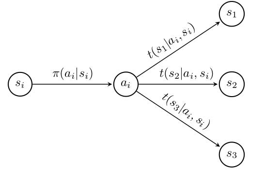](https://substackcdn.com/image/fetch/$s_!z7ER!,f_auto,q_auto:good,fl_progressive:steep/https%3A%2F%2Fsubstack-post-media.s3.amazonaws.com%2Fpublic%2Fimages%2Fc1fb9784-e12a-45eb-bf9e-c28ce1a9bf6e_547x354.png)
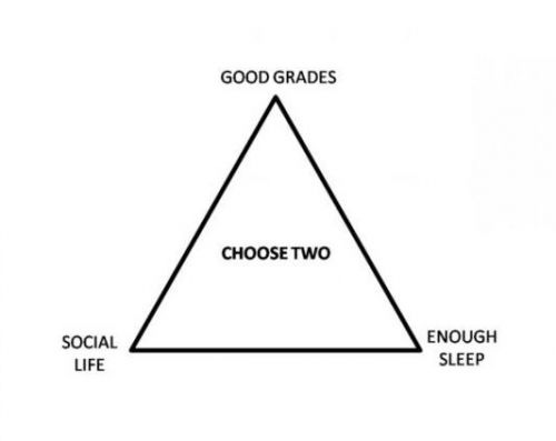
Using this structure, we would like to figure out what actions we should take to get the highest reward; fortunately, there exist proven algorithms to do exactly this\. We will soon attempt to solve for an optimal policy function π\(⋅\) using said algorithms in Markov’s world\. Through our specific example, we are attempting to solve the old, and suprisingly relevant meme \(below\), but with extreme precision due to the beauty of finite MDPs\.
[](https://substackcdn.com/image/fetch/$s_!npko!,f_auto,q_auto:good,fl_progressive:steep/https%3A%2F%2Fsubstack-post-media.s3.amazonaws.com%2Fpublic%2Fimages%2Fe36f205a-e89e-4f0b-9fc1-a66cb6509512_500x397.png)
Before, we reach the solution, however, we need a few more tools defined below\.
Given these well defined transition dynamics and rewards of Markov’s model world, we can define two additional functions\. The first is the state\-value function\. This is determined by the state Markov is currently in and also his current policy function:
\\\(v\_\\pi\(s\) = \\mathbb\{E\}\_\\pi\[\\Sigma\_\{k=0\}^\\infty \\gamma^kR\_\{t\+k\+1\}\|S\_t=s\]\\\)
This can be interpreted as the long\-term expected reward that Markov will receive from currently being in state sss and acting according to his plan\. Here, we have two random variables that*St*and*Rt*that model the state and reward the agent will be in and recieve, at time step*t*, if it follows the policy defined by π\(⋅\)\. We have also introduced a new variable γ which we call the discount rate, that can be any value from 0≤γ≤1\. The term in the expectation expands out to this form:
\\\(\\gamma^k R\_\{t\+k\+1\} = \\gamma^0 R\_1 \+ \\gamma^1 R\_2 \+ \\gamma^2 R\_3 \+ \\cdots\\\)
In essence, the value of the reward gained by taking an action and landing in a new state in the future, is being reduced by a multiple of γ with each time step that passes\. This answers the question on how much a given reward is depriciated each ttt time step into the future, before it has been obtained\.
Altogether, the state\-value function*vπ*\(⋅\) allows us to help Markov gauge the*value*he obtains from his tentative*plan*that we have formalized by the policy function*π\(⋅\)*\. Now, the curious Markov asks us, “Well, assume I’m working on my probability pset and decide to go read War and Peace by Leo Tolstoy, is that a good idea?” To answer this, let’s add our final function to put Markov’s mind at rest\. Let’s call it the action\-value function*qπ\(s,a\)*, which is the expected return in rewards he receives, computed similarly to the state\-value function, but incorporating the reward from an initial action aaa instead of action*π\(s\)*:
\\\(q\_\\pi\(s, a\) = \\mathbb\{E\}\_\\pi\[\\Sigma\_\{k=0\}^\\infty \\gamma^k R\_\{t\+k\+1\} \| S\_t = s, A\_t = a\]\\\)
This seemingly insignificant distinction will help us when it comes time to compute the optimal policy π*\**\(⋅\)\. Together, the state\-value and action\-value functions, are called the Bellman equations\. We, will now solve for the value of these Bellman equations at each state or state\-action pair, using two fundamental algorithms\.
The first main algorithm used to solve finite MDPs is called Policy Iteration\. This algorithm iterates between two steps\. The first step is to evaluate the value function for all states of an MDP given an arbitrary policy\. This is commonly referred to as*policy evaluation*\. The second step is to consider for each state, whether taking action a≠π\(s\) \(not part of the policy\) can improve the overall expected return\. This is commonly referred to as*policy evaluation*\. The algorithm loops through these steps, finding a better policy at each iteration until convergence\.
Now, we shall implement Markov’s model world using python and numpy\. We follow the standard algorithm implementation outlined in Richard Sutton’s RL[textbook](http://incompleteideas.net/book/first/ebook/node40.html)\. However, we make a few simplificiations for a quick build\. \(1\) Our model only has 1 reward per \(s’, s, a\) pairs, while others allow for a distribution over rewards \(2\) We are searching to solve for a deterministic policy, while others can solve for a stochastic policy \(3\) Instead of defining 56 carefully engineered rewards and transitions, we assign fixed values \(4\) To assure convergence of our expected long term reward \(to avoid values approaching infinity\), so we include a discount rate of 0\.85\.
We first need to make a few imports and initialize our finite MDP\.
```
import numpy as np
import matplotlib.pyplot as plt
import math
states = 3 #Number of States
actions = 3 #Number of Actions
rewards = 3 #Number of Rewards per State-action Pair
g = 0.85 #Discount Rate - gamma
v_s = [0, 0, 0] #State-value Function
pi = [0, 0, 0] #Deterministic Policy Function
theta = 1 #Hyperparameter
np.random.seed(0) #Random seed used to initalize Reward Function
R = 100 * np.random.rand(3, 3, 3) #Reward Function: intialize a 3x3x3 tensor of random values from 0 to 100
T = np.full((3,3,3), 1/3) #Transition Function: intialize a 3x3x3 tensor of 1/3s
PI = [] #List to keep track of value function for Policy Iteration
VI = [] #List to keep track of value function for Value Iteration
print(R) #Our specific Reward Function
#Randomly Initialized Reward Function
[[[54.88135039 71.51893664 60.27633761]
[54.4883183 42.36547993 64.58941131]
[43.75872113 89.17730008 96.36627605]]
[[38.34415188 79.17250381 52.88949198]
[56.80445611 92.55966383 7.10360582]
[ 8.71292997 2.02183974 83.26198455]]
[[77.81567509 87.00121482 97.86183422]
[79.91585642 46.14793623 78.05291763]
[11.82744259 63.99210213 14.33532874]]]
```
Now for the implementation of Policy Iteration, which initializes an arbitraty policy and state\-value function, then iterates between policy evaluation and policy improvement stages\.
```
def policy_iteration(pol, val, thres):
#Initialize Policy and Value Function
policy = pol
threshold = thres
v_s_init = val
PI.append(v_s_init.copy())
#Run first iteration of PE to evaluate your arbitrary policy
value = policy_evaluation(pi, v_s_init, threshold)
PI.append(value.copy())
#Run first iteration of PI to find actions that might prove it
policy_stable, policy = policy_improvement(pi, value)
#Repeat PE and PI, until no change in policy improves performance (i.e. policy_stable = True)
while policy_stable == False:
value = policy_evaluation(policy, value, threshold)
PI.append(value.copy())
policy_stable, policy = policy_improvement(policy, value)
return policy, value
def policy_evaluation(pol, val, thres):
policy = pol
threshold = thres
v_s_init = val
delta = math.inf
#Evalute accuracy until Delta drops below specified threshold value
while delta >= threshold:
delta = 0
#Compute expected return for each state, given the current policy
for s in range(states):
v = v_s_init[s]
E_r = 0
for s_p in range(states):
E_r += T[s, policy[s], s_p]*(R[s, policy[s], s_p] + g*v_s_init[s_p])
v_s_init[s] = E_r
delta = max(delta, abs(v - v_s_init[s]))
return v_s_init
def policy_improvement(pol, val):
policy_stable = True
policy = pol.copy()
v_s_init = val
for s in range(states):
old_a = pol[s]
v = v_s_init[s]
E_r = []
#Evalute expected value of each state and action pair
for a in range(actions):
e_r = 0
for s_p in range(states):
e_r += T[s, a, s_p]*(R[s, a, s_p] + g*v_s_init[s_p])
E_r.append(e_r)
#Select action the maximizes expected value
new_a = E_r.index(max(E_r))
#Compare if action that maximizes expected value is action specified by current policy
if(old_a != new_a):
#If not, modify policy and report stability to false, to ensure PI evalutes new policy
policy[s] = new_a
policy_stable = False
return policy_stable, policy
#Run Algorithm
new_pi, new_v = value_iteration(pi, v_s, theta)
```
Algorithm Output:
\\\(v\_\{\\pi\*\}\(s\_1, s\_2, s\_3\) = \[489\.98445020171096, 470\.622736297478, 501\.629766335168\]\\\)
\\\(\\pi\_\*\(s\_1, s\_2, s\_3\) = \[2, 0, 0\]\\\)
By running this algorithm, we obtain the optimal state\-value function and optimal policy shown above\. Now this example is clearly idealistic, we are given the states, actions, and rewards\. In the real world we don’t have this, and real world problems are typically much more complicated\. Figuring out how to solve more complex, obscure problems is an open challenge that the field faces to this day\. In short, MDPs solve real\-world problems only as best as you can model problems in the first place\. Therefore, although we may not be able gaurantee that our policy will help Markov in the real\-world, we hope that the theoretical implications can provide insight into his decision making\.
Now, let’s attempt to find the optimal policy of out student’s Markov’s work using Value Iteration\. The structure of this algorithm is very similar to Policy Iteration, but differs slightly\. Instead of iterating back and forth between improvement and evaluation in Policy Iteration, Value Iteration performs a single iteration of a pseudo policy evaluation, where it additionally sweeps over the action space and perform a max operation to return the optimal state\-value function and policy function upon completion\.
```
def value_iteration(pol, val, thres):
#Initialize Policy and Value Function
policy = pol
threshold = thres
v_s_init = val
VI.append(v_s_init.copy())
delta = math.inf
#Loop until delta reaches specified threshold
while delta >= threshold:
delta = 0
#Evalute expected value of each state and action pair
for s in range(states):
v = v_s_init[s]
E_r = []
for a in range(actions):
e_r = 0
for s_p in range(states):
e_r += T[s, a, s_p]*(R[s, a, s_p] + g*v_s_init[s_p])
E_r.append(e_r)
#Update policy with action that maximizes return
policy[s] = E_r.index(max(E_r))
#Update new state-value function accordingly
v_s_init[s] = max(E_r)
delta = max(delta, abs(v - v_s_init[s]))
I.append(v_s_init.copy())
return policy, v_s_init
#Run Algorithm
new_pi, new_v = value_iteration(pi, v_s, theta)
```
Algorithm Ouput:
\\\(v\_\{\\pi\*\}\(s\_1, s\_2, s\_3\) = \[490\.2756261387957, 470\.8914747627405, 501\.8777964782847\]\\\)
\\\(\\pi\_\*\(s\_1, s\_2, s\_3\) = \[2, 0, 0\]\\\)
By running this algorithm, we obtain the optimal state\-value function and optimal policy shown above\. Overall, both methods follow different paths to reach the same solution, each carefully designed to use the Bellman equations to better understand the MDP\.
This blog only covers the basics, and there is much more to explore in MDP theory\. For example, there exists many extensions and generalizations to this framework, such as the partially observed or continous cases, studied by mathematicians and engineers alike\. If this blog interested you and you want to dive deeper into algorithms for solving finite, discrete markov chains, then take a look at the references for a more detailed treatment of the topic\.
- Introduction in Reinforcment Learning by Sutton and Barto, Chapters 3 and 4\*
- Probability in Electrical Engineering and Computer Science by Jean Walrand, Chapters 11 and 12
- Dynamic Programming and Markov Processes by Ronald Howard
- [https://en\.wikipedia\.org/wiki/Deep\_reinforcement\_learning](https://en.wikipedia.org/wiki/Deep_reinforcement_learning)
- [https://en\.wikipedia\.org/wiki/Markov\_decision\_process](https://en.wikipedia.org/wiki/Markov_decision_process)
- [http://incompleteideas\.net/](http://incompleteideas.net/)
- Read Bibliographical and Historial Remarks for a deeper dive
- [https://web\.stanford\.edu/class/cme241/lecture\_slides/rich\_sutton\_slides/5\-6\-MDPs\.pdf](https://web.stanford.edu/class/cme241/lecture_slides/rich_sutton_slides/5-6-MDPs.pdf)
- [https://inst\.eecs\.berkeley\.edu/~cs188/sp20/assets/lecture/lec10\.pdf](https://inst.eecs.berkeley.edu/~cs188/sp20/assets/lecture/lec10.pdf)
- [https://people\.eecs\.berkeley\.edu/~pabbeel/cs287\-fa12/slides/mdps\-exact\-methods\.pdf](https://people.eecs.berkeley.edu/~pabbeel/cs287-fa12/slides/mdps-exact-methods.pdf)
- [https://people\.eecs\.berkeley\.edu/~pabbeel/cs287\-fa12/](https://people.eecs.berkeley.edu/~pabbeel/cs287-fa12/)
- [https://www\.cse\.iitb\.ac\.in/~shivaram/resources/ijcai\-2017\-tutorial\-policyiteration/tapi\.pdf](https://www.cse.iitb.ac.in/~shivaram/resources/ijcai-2017-tutorial-policyiteration/tapi.pdf)
- [https://homes\.cs\.washington\.edu/~todorov//courses/amath579/MDP\.pdf](https://homes.cs.washington.edu/~todorov//courses/amath579/MDP.pdf)
- [https://www\.tau\.ac\.il/~mansour/rl\.html](https://www.tau.ac.il/~mansour/rl.html)
- [https://www\.cs\.mcgill\.ca/~dprecup/courses/AI/Lectures/ai\-lecture16\.pdf](https://www.cs.mcgill.ca/~dprecup/courses/AI/Lectures/ai-lecture16.pdf)
- [https://en\.wikipedia\.org/wiki/Markov\_decision\_process\#Extensions\_and\_generalizations](https://en.wikipedia.org/wiki/Markov_decision_process#Extensions_and_generalizations)
- [https://arxiv\.org/pdf/1302\.4971\.pdf](https://arxiv.org/pdf/1302.4971.pdf)
- [http://incompleteideas\.net/RandomMDPs\.html](http://incompleteideas.net/RandomMDPs.html)
- [https://www\.youtube\.com/watch?v=vY\-voHb22io&list=PLKlhhkvvU8\-aXmPQZNYG\_e\-2nTd0tJE8v&index=35&t=0s](https://www.youtube.com/watch?v=vY-voHb22io&list=PLKlhhkvvU8-aXmPQZNYG_e-2nTd0tJE8v&index=35&t=0s)
##### Other Blogs
- [https://towardsdatascience\.com/introduction\-to\-reinforcement\-learning\-markov\-decision\-process\-44c533ebf8da](https://towardsdatascience.com/introduction-to-reinforcement-learning-markov-decision-process-44c533ebf8da)\(3 part series\)
#### Discussion about this post
### Ready for more?
Introduces a novel shielding framework for robust Markov decision processes (RMDPs) that formally guarantees safety under uncertain transition dynamics, proving soundness and optimality. The approach combines with PAC guarantees for learned models, enabling safe reinforcement learning in unknown environments.
This paper introduces adaptive probabilistic shielding for safe reinforcement learning, where the shield is computed from an online learned MDP model, adapting as the model becomes more accurate.
Progressive Point Matching (PPM) is a framework proposed to assign partial credit in reinforcement learning for long-horizon tasks in LLMs, addressing the inefficiency of sparse outcome rewards by treating reasoning as paths through a Markovian state space.
This paper formalizes the sim-to-real gap for foundation model agents as a Markov Decision Process problem, proposing a unified research agenda to adapt classical solutions like domain randomization for improving agent robustness and reliability in real-world deployment.
This paper introduces a property-driven causal abstraction technique for factored Markov Decision Processes (MDPs), grouping states based on causal relations over state variable predicates to reduce model size while preserving property-relevant behavior. The approach is evaluated on standard benchmarks, yielding small abstractions that support near-optimal policy computation and often generalize to larger MDPs.