This article explains how to compute closing speed as the normal component of relative velocity between two objects using vector projection, with examples for physics simulations and game engines.
<p>In Physics simulations or game engines it’s sometimes useful to
determine the speed with which two objects are approaching each other.
This post will discuss the concept of <em>closing speed</em>, which is the
<em>normal component</em> of the <em>relative velocity</em> of two objects.</p>
<div class="section" id="relative-velocity-and-its-components">
<h2>Relative velocity and its components</h2>
<p>Suppose we have objects A and B <a class="footnote-reference" href="#footnote-1" id="footnote-reference-1">[1]</a> with velocity vectors
<object class="valign-m3 latex-math" data="https://eli.thegreenplace.net/images/math/94a17f930633898bbe6d1ef2a6c263573aa3842a.svg" style="height: 20px;" type="image/svg+xml">\vec{V_A}</object> and <object class="valign-m3 latex-math" data="https://eli.thegreenplace.net/images/math/c4f87fb6f28657fbd625b4bfbc514b0574e80108.svg" style="height: 20px;" type="image/svg+xml">\vec{V_B}</object>. The <em>relative velocity</em> of B
w.r.t. A is:</p>
<object class="align-center" data="https://eli.thegreenplace.net/images/math/27625ffaa87e60a1f991ed3aa390d5b284868118.svg" style="height: 24px;" type="image/svg+xml">\[\vec{V}_{B|A}=\vec{V}_B-\vec{V}_A\]</object>
<p>Put differently, it’s the velocity of B in A’s frame of reference.</p>
<p>This relative velocity is a vector, and we can split it into orthogonal
components. Obviously, the nature of such a split depends on the basis
we want to use. We could look at the vector’s x an y components (we’ll
be using <img alt="\mathbb{R}^2" class="valign-0 latex-math" src="https://eli.thegreenplace.net/images/math/2b688757b3d0949451e1fa97e71ac5f5f284a5e4.png" style="height: 15px;" /> - two dimensional space, but everything
here applies to 3D as well), but for this post we’re interested in
something slightly different:</p>
<img alt="Normal and tangential components of the relative velocity." class="align-center" src="https://eli.thegreenplace.net/images/2026/normal-and-tangential.png" />
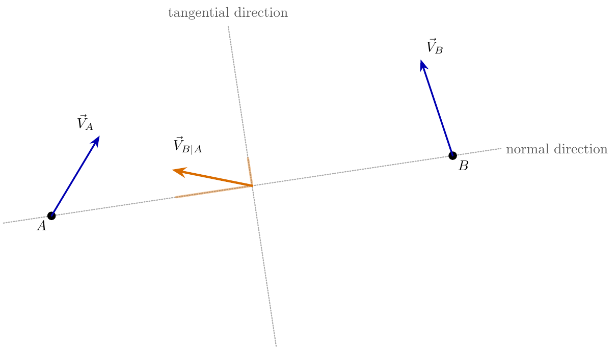
<p>We draw a line connecting the two objects. The component of
<object class="valign-m6 latex-math" data="https://eli.thegreenplace.net/images/math/8ccc4a9163c92ed1e8e723b64a9d7056ada65491.svg" style="height: 24px;" type="image/svg+xml">\vec{V}_{B|A}</object> in the direction of this line is called the
<em>normal component</em> of relative velocity, while the component
perpendicular to this direction is called the <em>tangential component</em>.</p>
</div>
<div class="section" id="computing-the-normal-component">
<h2>Computing the normal component</h2>
<p>How do we find the component of a vector in the direction of a specific
line? By using a <a class="reference external" href="https://eli.thegreenplace.net/2024/projections-and-projection-matrices/">vector
projection!</a>.
We’ll represent the line by a vector, and find the projection of
<object class="valign-m6 latex-math" data="https://eli.thegreenplace.net/images/math/8ccc4a9163c92ed1e8e723b64a9d7056ada65491.svg" style="height: 24px;" type="image/svg+xml">\vec{V}_{B|A}</object> onto this vector.</p>
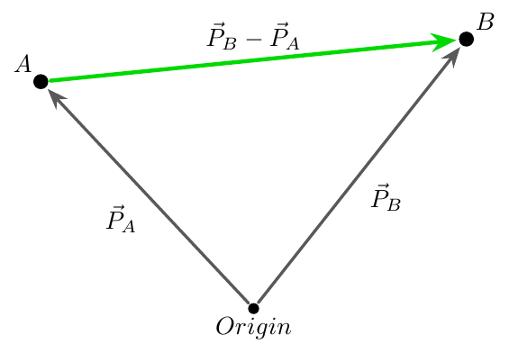
<p>The positions of A and B can also be seen as vectors: <object class="valign-m3 latex-math" data="https://eli.thegreenplace.net/images/math/0cbd4a39e2dc15c143419b61cfab3d08c89dd946.svg" style="height: 20px;" type="image/svg+xml">\vec{P}_A</object>
and <object class="valign-m3 latex-math" data="https://eli.thegreenplace.net/images/math/8be98601c153883b6091b8ba841746479c876b9c.svg" style="height: 20px;" type="image/svg+xml">\vec{P}_B</object>. The line connecting them can then be expressed as
the vector <object class="valign-m3 latex-math" data="https://eli.thegreenplace.net/images/math/702505a802f90f2627da0f341f6f28af8a4a2aca.svg" style="height: 20px;" type="image/svg+xml">\vec{P}_B-\vec{P}_A</object>:</p>
<img alt="The relative-position vector is the difference of the two position vectors." class="align-center" src="https://eli.thegreenplace.net/images/2026/the-relative-position.png" />
<p>All we need from this position difference vector is its direction, not
its magnitude, however <a class="footnote-reference" href="#footnote-2" id="footnote-reference-2">[2]</a>. So we’ll use the <em>unit vector</em> of
<object class="valign-m3 latex-math" data="https://eli.thegreenplace.net/images/math/702505a802f90f2627da0f341f6f28af8a4a2aca.svg" style="height: 20px;" type="image/svg+xml">\vec{P}_B-\vec{P}_A</object>, denoted as:</p>
<object class="align-center" data="https://eli.thegreenplace.net/images/math/4037effd91b348b652473f482fc242b7dc83ea57.svg" style="height: 49px;" type="image/svg+xml">\[\widehat{P}=\frac{\vec{P}_B-\vec{P}_A}{|\vec{P}_B-\vec{P}_A|}\]</object>
<p>Finally, to find the projection of <object class="valign-m6 latex-math" data="https://eli.thegreenplace.net/images/math/8ccc4a9163c92ed1e8e723b64a9d7056ada65491.svg" style="height: 24px;" type="image/svg+xml">\vec{V}_{B|A}</object> onto
<object class="valign-0 latex-math" data="https://eli.thegreenplace.net/images/math/ae76f98aa161c8e6255ff6aac4741c7745715b54.svg" style="height: 17px;" type="image/svg+xml">\widehat{P}</object>, we compute <a class="footnote-reference" href="#footnote-3" id="footnote-reference-3">[3]</a>:</p>
<object class="align-center" data="https://eli.thegreenplace.net/images/math/bfa87afcdbc16f27582886265e68c81a888a5719.svg" style="height: 24px;" type="image/svg+xml">\[S_c=\vec{V}_{B|A}\cdot\widehat{P}=(\vec{V}_B-\vec{V}_A)\cdot\widehat{P}\]</object>
<p>Where the multiplication operator between the vectors is the <em>dot
product</em>. Note that the result of the dot product is a scalar;
therefore, the quantity <object class="valign-m3 latex-math" data="https://eli.thegreenplace.net/images/math/b423d57e7c978d9b6f9e3d76c3e02f52cf5a1a17.svg" style="height: 15px;" type="image/svg+xml">S_c</object> is called the <em>closing speed</em> - it
expresses the rate at which the relative distance of the two objects is
changing. If it’s positive, the objects are drifting farther apart; if
it’s negative, the objects are getting closer together. Therefore the
term "closing speed" may be slightly confusing; alternatively, this has
been called a "signed separation speed", or "normal relative speed" <a class="footnote-reference" href="#footnote-4" id="footnote-reference-4">[4]</a>.</p>
<p>The signs in these calculations can be tricky to get right, so we have
to be very careful. Let’s see a few examples that will help us make
these computations more concrete.</p>
</div>
<div class="section" id="examples">
<h2>Examples</h2>
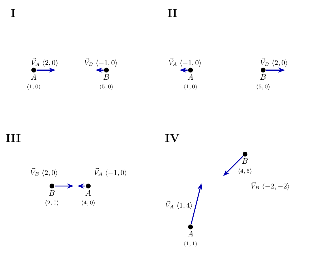
<p>To build up some intuition and get some practice with the equations,
we’ll review the following examples:</p>
<img alt="Four relative-motion examples." class="align-center" src="https://eli.thegreenplace.net/images/2026/four-relative-motion.png" />
<p><strong>Example I</strong>: We’ll start by computing the relative position unit
vector <object class="valign-0 latex-math" data="https://eli.thegreenplace.net/images/math/ae76f98aa161c8e6255ff6aac4741c7745715b54.svg" style="height: 17px;" type="image/svg+xml">\widehat{P}</object>:</p>
<object class="align-center" data="https://eli.thegreenplace.net/images/math/f28d4a7d06cafd403cd826c0a670975b172ff67a.svg" style="height: 49px;" type="image/svg+xml">\[\widehat{P}=\frac{\vec{P}_B-\vec{P}_A}{|\vec{P}_B-\vec{P}_A|}=\frac{\langle 4,0\rangle}{|\langle 4,0 \rangle|}=\langle1,0\rangle\]</object>
<p>Then, the closing speed is:</p>
<object class="align-center" data="https://eli.thegreenplace.net/images/math/f3b2874b8233cd8c1751ed5ff2fdfbae1d96c711.svg" style="height: 22px;" type="image/svg+xml">\[S_c=(\vec{V}_B-\vec{V}_A)\cdot\widehat{P}=\langle -3,0\rangle\cdot\langle1,0\rangle=-3\]</object>
<p>Based on our convention, the negative sign of <object class="valign-m3 latex-math" data="https://eli.thegreenplace.net/images/math/b423d57e7c978d9b6f9e3d76c3e02f52cf5a1a17.svg" style="height: 15px;" type="image/svg+xml">S_c</object> means that the
objects are approaching each other. Due to the simple nature of the
example, this result is easy to verify, as it can be immediately guessed
just by looking at the diagram.</p>
<p><strong>Example II</strong>: Here <object class="valign-0 latex-math" data="https://eli.thegreenplace.net/images/math/ae76f98aa161c8e6255ff6aac4741c7745715b54.svg" style="height: 17px;" type="image/svg+xml">\widehat{P}</object> is the same as in the previous
example. The closing speed is:</p>
<object class="align-center" data="https://eli.thegreenplace.net/images/math/f66ddd84100e0b1eaafe03b3afed57dc50a82965.svg" style="height: 22px;" type="image/svg+xml">\[S_c=(\vec{V}_B-\vec{V}_A)\cdot\widehat{P}=\langle 3,0\rangle\cdot\langle1,0\rangle=3\]</object>
<p>Same magnitude, but different sign from before, because the objects are
moving farther apart.</p>
<p><strong>Example III</strong> This example is to demonstrate that we get consistent
results even if B is to the left of A. Here the relative position unit
vector is:</p>
<object class="align-center" data="https://eli.thegreenplace.net/images/math/e7796cd9ca52dc9cf7de0692372020ef2303bbb8.svg" style="height: 49px;" type="image/svg+xml">\[\widehat{P}=\frac{\vec{P}_B-\vec{P}_A}{|\vec{P}_B-\vec{P}_A|}=\frac{\langle -2,0\rangle}{|\langle -2,0 \rangle|}=\langle-1,0\rangle\]</object>
<p>And the closing speed:</p>
<object class="align-center" data="https://eli.thegreenplace.net/images/math/67c72205da69531f03dd92be8d75a04c775e5342.svg" style="height: 22px;" type="image/svg+xml">\[S_c=(\vec{V}_B-\vec{V}_A)\cdot\widehat{P}=\langle 3,0\rangle\cdot\langle -1,0\rangle=-3\]</object>
<p>Which is the same as in example I, as expected. The direction of
<object class="valign-0 latex-math" data="https://eli.thegreenplace.net/images/math/ae76f98aa161c8e6255ff6aac4741c7745715b54.svg" style="height: 17px;" type="image/svg+xml">\widehat{P}</object> flipped, but so did the direction of the relative
velocity vector, so the result has the same sign.</p>
<p><strong>Example IV</strong>: Finally, an example showing more arbitrary positions and
velocities.</p>
<object class="align-center" data="https://eli.thegreenplace.net/images/math/aa10ecf2964b6bfc8fc7613fe86515408c2fa555.svg" style="height: 49px;" type="image/svg+xml">\[\widehat{P}=\frac{\vec{P}_B-\vec{P}_A}{|\vec{P}_B-\vec{P}_A|}=\frac{\langle 3,4\rangle}{|\langle 3,4 \rangle|}=\langle0.6,0.8\rangle\]</object>
<p>Then:</p>
<object class="align-center" data="https://eli.thegreenplace.net/images/math/a03119506d85247140be836d2e7c898ba991e46e.svg" style="height: 22px;" type="image/svg+xml">\[S_c=(\vec{V}_B-\vec{V}_A)\cdot\widehat{P}=\langle -3,-6\rangle\cdot\langle 0.6,0.8\rangle=-6.6\]</object>
<p>This example is a good opportunity to demonstrate something important
about <object class="valign-m3 latex-math" data="https://eli.thegreenplace.net/images/math/b423d57e7c978d9b6f9e3d76c3e02f52cf5a1a17.svg" style="height: 15px;" type="image/svg+xml">S_c</object>: it’s time-dependent, because positions change with
time. Here, -6.6 is the closing speed at the exact moment when A’s and
B’s positions and velocities are as stated in the example. In the next
time step, the position of A will be <object class="valign-m4 latex-math" data="https://eli.thegreenplace.net/images/math/2bc27b863835e60fdba1357f797159dc72d77045.svg" style="height: 18px;" type="image/svg+xml">\langle2,5\rangle</object> and the
position of B will be <object class="valign-m4 latex-math" data="https://eli.thegreenplace.net/images/math/2450a84c29d863591b7db00ceada4f084bfb99ea.svg" style="height: 18px;" type="image/svg+xml">\langle2,3\rangle</object>, while their velocities
remain the same. The <object class="valign-m3 latex-math" data="https://eli.thegreenplace.net/images/math/b423d57e7c978d9b6f9e3d76c3e02f52cf5a1a17.svg" style="height: 15px;" type="image/svg+xml">S_c</object> then will be quite different. This is a
good segue to the next topic - which is a more physical view of closing
speed.</p>
</div>
<div class="section" id="closing-speed-as-a-function-of-time">
<h2>Closing speed as a function of time</h2>
<p>The computation shown so far represents a static view of the world;
perhaps the right word to use is <em>instantaneous</em>. Given the positions
and velocities at a given moment, what is the closing speed between the
objects <em>at that exact moment</em>?</p>
<p>But there’s no reason to not generalize this using a more standard
physical interpretation of velocity.</p>
<p>First, let’s state the position vectors of A and B as a function of
time: <object class="valign-m4 latex-math" data="https://eli.thegreenplace.net/images/math/4eb67887f180834938958d847a67ce8c4e833101.svg" style="height: 22px;" type="image/svg+xml">\vec{P}_A(t)</object> and <object class="valign-m4 latex-math" data="https://eli.thegreenplace.net/images/math/3b69a9ddd6f52dba77380fd33edf1ce5adb8e57d.svg" style="height: 22px;" type="image/svg+xml">\vec{P}_B(t)</object>. The relative
position vector between the objects is also a function of time:</p>
<object class="align-center" data="https://eli.thegreenplace.net/images/math/70dfcf594bc9407384d7c009f9a608eb3fef4e73.svg" style="height: 22px;" type="image/svg+xml">\[\vec{R}(t)=\vec{P}_B(t)-\vec{P}_A(t)\]</object>
<p>Now we’ll define the scalar distance as the magnitude of this vector:</p>
<object class="align-center" data="https://eli.thegreenplace.net/images/math/7cdc889c6f871266456a41fba1c39755e176be60.svg" style="height: 22px;" type="image/svg+xml">\[r(t)=|\vec{R}(t)|=|\vec{P}_B(t)-\vec{P}_A(t)|\]</object>
<p>We’re interested in <object class="valign-m6 latex-math" data="https://eli.thegreenplace.net/images/math/2e486b6ff05146a7eec038ad6e7e0fc8528811c3.svg" style="height: 24px;" type="image/svg+xml">\frac{dr(t)}{dt}</object> - the change in this
distance over time. Let’s start by breaking <object class="valign-m4 latex-math" data="https://eli.thegreenplace.net/images/math/9f99e0576aed540806bce0791e5746726e6e413e.svg" style="height: 18px;" type="image/svg+xml">R(t)</object> down to its
constituents:</p>
<object class="align-center" data="https://eli.thegreenplace.net/images/math/f3fe85228247cba64b2cf42ab620ca2ad021f58e.svg" style="height: 51px;" type="image/svg+xml">\[\begin{aligned}
\vec{R}(t)&=\langle x(t),y(t)\rangle \\
r(t)&=\sqrt{x(t)^2+y(t)^2}
\end{aligned}\]</object>
<p>By the chain rule <a class="footnote-reference" href="#footnote-5" id="footnote-reference-5">[5]</a>:</p>
<object class="align-center" data="https://eli.thegreenplace.net/images/math/6306fb3b34832bfa2973b4f5f2ce022e50e61bfc.svg" style="height: 100px;" type="image/svg+xml">\[\begin{aligned}
\frac{dr(t)}{dt}&=\frac{\frac{d}{dt}(x(t)^2+y(t)^2)}{2\sqrt{x(t)^2+y(t)^2}}\\
&=\frac{2x(t)x'(t)+2y(t)y'(t)}{2\sqrt{x(t)^2+y(t)^2}}
=\frac{x(t)x'(t)+y(t)y'(t)}{\sqrt{x(t)^2+y(t)^2}}
\end{aligned}\]</object>
<p>Switching back to the vector representation: since
<object class="valign-m4 latex-math" data="https://eli.thegreenplace.net/images/math/07a18a0fb49fd212904167765ad6d84a0c82e087.svg" style="height: 22px;" type="image/svg+xml">\vec{R}(t)=\langle x(t),y(t)\rangle</object>, the numerator of the
fraction above is then a dot product between <object class="valign-m4 latex-math" data="https://eli.thegreenplace.net/images/math/7c50f292ef65e21556b433d72d5c11b6e9f87ecf.svg" style="height: 22px;" type="image/svg+xml">\vec{R}(t)</object> and
<object class="valign-m4 latex-math" data="https://eli.thegreenplace.net/images/math/4dfa75b6830d41bca1c17cdb195e628f68ed338b.svg" style="height: 22px;" type="image/svg+xml">\vec{R}'(t)</object>, we can write this as:</p>
<object class="align-center" data="https://eli.thegreenplace.net/images/math/a42dd678ac96ed753c3c3526680198572a2fe257.svg" style="height: 49px;" type="image/svg+xml">\[\frac{dr(t)}{dt}=\frac{\vec{R}(t)\cdot\vec{R}'(t)}{|\vec{R}(t)|}=\hat{R}(t)\cdot\vec{R}'(t)\]</object>
<p>But <object class="valign-m4 latex-math" data="https://eli.thegreenplace.net/images/math/54361db0be49009bd9ab092a77a7a00ddf8a1639.svg" style="height: 21px;" type="image/svg+xml">\hat{R}(t)</object> is precisely <object class="valign-0 latex-math" data="https://eli.thegreenplace.net/images/math/1787f35be0deea91d648e299fd551f3dcb3e44b5.svg" style="height: 17px;" type="image/svg+xml">\hat{P}</object> from the earlier
section, as a function of time. Moreover:</p>
<object class="align-center" data="https://eli.thegreenplace.net/images/math/a98048e9ed9db3cf9b4799aa6f6146b7dd2cb992.svg" style="height: 22px;" type="image/svg+xml">\[\vec{R}'(t)=\vec{P}'_B(t)-\vec{P}'_A(t)=\vec{V}_B(t)-\vec{V}_A(t)\]</object>
<p>Because velocity is the time derivative of position. Therefore, we end
up with the same equation, just as a function of time:</p>
<object class="align-center" data="https://eli.thegreenplace.net/images/math/e3e0da99f86f0ff329cba714e12223664276b75c.svg" style="height: 38px;" type="image/svg+xml">\[\frac{dr(t)}{dt}=\hat{P}(t)\cdot(\vec{V}_B(t)-\vec{V}_A(t))\]</object>
<p>This formulation is more precise because it makes it very obvious that
all the quantities we’re dealing with are time dependent.</p>
<hr class="docutils" />
<table class="docutils footnote" frame="void" id="footnote-1" rules="none">
<colgroup><col class="label" /><col /></colgroup>
<tbody valign="top">
<tr><td class="label"><a class="fn-backref" href="#footnote-reference-1">[1]</a></td><td>Throughout this post, we assume our objects are sufficiently far
apart that they can be treated as <em>points</em> (or <em>particles</em>) without
any shape, area or volume.</td></tr>
</tbody>
</table>
<table class="docutils footnote" frame="void" id="footnote-2" rules="none">
<colgroup><col class="label" /><col /></colgroup>
<tbody valign="top">
<tr><td class="label"><a class="fn-backref" href="#footnote-reference-2">[2]</a></td><td>The velocity components should be the same regardless of how far
apart the two objects are.</td></tr>
</tbody>
</table>
<table class="docutils footnote" frame="void" id="footnote-3" rules="none">
<colgroup><col class="label" /><col /></colgroup>
<tbody valign="top">
<tr><td class="label"><a class="fn-backref" href="#footnote-reference-3">[3]</a></td><td>In the standard projection formula we’d also divide by the magnitude
of <object class="valign-0 latex-math" data="https://eli.thegreenplace.net/images/math/ae76f98aa161c8e6255ff6aac4741c7745715b54.svg" style="height: 17px;" type="image/svg+xml">\widehat{P}</object>, but in our case it’s a unit vector anyway.</td></tr>
</tbody>
</table>
<table class="docutils footnote" frame="void" id="footnote-4" rules="none">
<colgroup><col class="label" /><col /></colgroup>
<tbody valign="top">
<tr><td class="label"><a class="fn-backref" href="#footnote-reference-4">[4]</a></td><td>In some online sources you may see the closing speed described as
closing velocity because it has a direction. IMHO this is the wrong
framing. Scalars can be signed! The closing speed is certainly a
scalar, not a vector.</td></tr>
</tbody>
</table>
<table class="docutils footnote" frame="void" id="footnote-5" rules="none">
<colgroup><col class="label" /><col /></colgroup>
<tbody valign="top">
<tr><td class="label"><a class="fn-backref" href="#footnote-reference-5">[5]</a></td><td>The notation <object class="valign-m4 latex-math" data="https://eli.thegreenplace.net/images/math/8cef7d030134448b059cf3ccf9ef9edc29b769c0.svg" style="height: 18px;" type="image/svg+xml">x'(t)</object> means <object class="valign-m6 latex-math" data="https://eli.thegreenplace.net/images/math/153450414b2add185e4ad0b5fe515c2835446bfe.svg" style="height: 24px;" type="image/svg+xml">\frac{dx(t)}{dt}</object></td></tr>
</tbody>
</table>
</div>
# Relative velocity and closing speed
Source: [https://eli.thegreenplace.net/2026/relative-velocity-and-closing-speed](https://eli.thegreenplace.net/2026/relative-velocity-and-closing-speed)
In Physics simulations or game engines it’s sometimes useful to determine the speed with which two objects are approaching each other\. This post will discuss the concept of*closing speed*, which is the*normal component*of the*relative velocity*of two objects\.
## Relative velocity and its components
Suppose we have objects A and B[\[1\]](https://eli.thegreenplace.net/2026/relative-velocity-and-closing-speed#footnote-1)with velocity vectors and \. The*relative velocity*of B w\.r\.t\. A is:
Put differently, it’s the velocity of B in A’s frame of reference\.
This relative velocity is a vector, and we can split it into orthogonal components\. Obviously, the nature of such a split depends on the basis we want to use\. We could look at the vector’s x an y components \(we’ll be using\- two dimensional space, but everything here applies to 3D as well\), but for this post we’re interested in something slightly different:
We draw a line connecting the two objects\. The component of in the direction of this line is called the*normal component*of relative velocity, while the component perpendicular to this direction is called the*tangential component*\.
## Computing the normal component
How do we find the component of a vector in the direction of a specific line? By using a[vector projection\!](https://eli.thegreenplace.net/2024/projections-and-projection-matrices/)\. We’ll represent the line by a vector, and find the projection of onto this vector\.
The positions of A and B can also be seen as vectors: and \. The line connecting them can then be expressed as the vector :
All we need from this position difference vector is its direction, not its magnitude, however[\[2\]](https://eli.thegreenplace.net/2026/relative-velocity-and-closing-speed#footnote-2)\. So we’ll use the*unit vector*of , denoted as:
Finally, to find the projection of onto , we compute[\[3\]](https://eli.thegreenplace.net/2026/relative-velocity-and-closing-speed#footnote-3):
Where the multiplication operator between the vectors is the*dot product*\. Note that the result of the dot product is a scalar; therefore, the quantity is called the*closing speed*\- it expresses the rate at which the relative distance of the two objects is changing\. If it’s positive, the objects are drifting farther apart; if it’s negative, the objects are getting closer together\. Therefore the term "closing speed" may be slightly confusing; alternatively, this has been called a "signed separation speed", or "normal relative speed"[\[4\]](https://eli.thegreenplace.net/2026/relative-velocity-and-closing-speed#footnote-4)\.
The signs in these calculations can be tricky to get right, so we have to be very careful\. Let’s see a few examples that will help us make these computations more concrete\.
## Examples
To build up some intuition and get some practice with the equations, we’ll review the following examples:
**Example I**: We’ll start by computing the relative position unit vector :
Then, the closing speed is:
Based on our convention, the negative sign of means that the objects are approaching each other\. Due to the simple nature of the example, this result is easy to verify, as it can be immediately guessed just by looking at the diagram\.
**Example II**: Here is the same as in the previous example\. The closing speed is:
Same magnitude, but different sign from before, because the objects are moving farther apart\.
**Example III**This example is to demonstrate that we get consistent results even if B is to the left of A\. Here the relative position unit vector is:
And the closing speed:
Which is the same as in example I, as expected\. The direction of flipped, but so did the direction of the relative velocity vector, so the result has the same sign\.
**Example IV**: Finally, an example showing more arbitrary positions and velocities\.
Then:
This example is a good opportunity to demonstrate something important about : it’s time\-dependent, because positions change with time\. Here, \-6\.6 is the closing speed at the exact moment when A’s and B’s positions and velocities are as stated in the example\. In the next time step, the position of A will be and the position of B will be , while their velocities remain the same\. The then will be quite different\. This is a good segue to the next topic \- which is a more physical view of closing speed\.
## Closing speed as a function of time
The computation shown so far represents a static view of the world; perhaps the right word to use is*instantaneous*\. Given the positions and velocities at a given moment, what is the closing speed between the objects*at that exact moment*?
But there’s no reason to not generalize this using a more standard physical interpretation of velocity\.
First, let’s state the position vectors of A and B as a function of time: and \. The relative position vector between the objects is also a function of time:
Now we’ll define the scalar distance as the magnitude of this vector:
We’re interested in \- the change in this distance over time\. Let’s start by breaking down to its constituents:
By the chain rule[\[5\]](https://eli.thegreenplace.net/2026/relative-velocity-and-closing-speed#footnote-5):
Switching back to the vector representation: since , the numerator of the fraction above is then a dot product between and , we can write this as:
But is precisely from the earlier section, as a function of time\. Moreover:
Because velocity is the time derivative of position\. Therefore, we end up with the same equation, just as a function of time:
This formulation is more precise because it makes it very obvious that all the quantities we’re dealing with are time dependent\.
---
[\[1\]](https://eli.thegreenplace.net/2026/relative-velocity-and-closing-speed#footnote-reference-1)Throughout this post, we assume our objects are sufficiently far apart that they can be treated as*points*\(or*particles*\) without any shape, area or volume\.[\[2\]](https://eli.thegreenplace.net/2026/relative-velocity-and-closing-speed#footnote-reference-2)The velocity components should be the same regardless of how far apart the two objects are\.[\[3\]](https://eli.thegreenplace.net/2026/relative-velocity-and-closing-speed#footnote-reference-3)In the standard projection formula we’d also divide by the magnitude of , but in our case it’s a unit vector anyway\.[\[4\]](https://eli.thegreenplace.net/2026/relative-velocity-and-closing-speed#footnote-reference-4)In some online sources you may see the closing speed described as closing velocity because it has a direction\. IMHO this is the wrong framing\. Scalars can be signed\! The closing speed is certainly a scalar, not a vector\.[\[5\]](https://eli.thegreenplace.net/2026/relative-velocity-and-closing-speed#footnote-reference-5)The notation means
A combat game demo built with Claude Fable where the speed of light is artificially slowed, creating relativistic visual effects like light delay and aberration. The implementation uses a vertex shader with camera pose history to compute retarded positions per vertex.
The article focuses on relativistic raytracing, a technique that combines raytracing with relativistic physics to improve simulation accuracy in computer graphics and scientific visualization.
Niantic Spatial, Flexion, and NVIDIA demonstrate a sim2real pipeline for humanoid robots using digital twins and RL, achieving zero-shot transfer from simulation to real office navigation.
This article explains the fundamental mathematics of 3D to 2D projection in graphics, focusing on depth division and the perspective projection matrix, with practical examples.
PhysiFormer uses coordinate-space diffusion to generate physically-plausible 3D object motions without explicit inductive biases, enabling efficient multi-object reasoning and generalization to complex materials and geometries.